These models often need to be applied at scale, so large ensembles aren’t encouraged. To incentivise more lightweight solutions, we are adding an additional submission criteria: your submission should take a reasonable time to train and run inference. Specifically, we should be able to re-create your submission on a single-GPU machine (eg Nvidia P100) with less than 8 hours training and two hours inference.

Fields are each assigned a unique Field_ID. For the training set, you are provided the year the data was collected, the ‘label quality’ and the yield in UNITS. For the test set, you must estimate the yield based on the satellite data.

Field locations were collected by recording the GPS position during data capture. However, not all recorded positions fall within fields - some were recorded at the edge of the field (small offset error) while others were erroneously recorded in entirely separate locations, usually in built-up areas. To help combat this, we’ve manually reviewed some of these locations and assigned them a ’Quality’. ‘Good’ quality locations are obviously within a single field. ‘Medium’ quality locations were near a field, and the location has been adjusted to lie closer to the center of that field. And ‘Poor’ quality locations have no obvious field associated with them - you will likely wish to exclude these.

The test set consists entirely of fields whose location was considered ‘Good’ or ‘Medium’ by our labelling team.

For each field, you are given an image time series centered on the recorded field position. For each month, bands from two main sources (S2 and TERRACLIM) are included.

There are 30 bands for each of 12 months, giving a total of 360 image bands. The band names are provided in the bandnames.txt file in the form: MONTH_SOURCE_BANDNAME

For example, 0_S2_B4 is the RED (band 4) band of a Sentinel 2 image from January the year the data for this field was collected.

The imagery is all presented at 10m resolution, and the image is 41px a side. The center (im[20, 20]) is the field location.

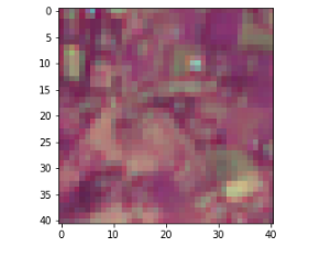
The starter notebook shows how to load the data for a given location into a numpy array, and how to plot the visible bands from a given month to create an image like the following:

Sentinel 2 images are collected more than once a month - to generate the inputs for this challenge the least cloudy image from each month was used.

No external data is permitted for this competition, and thus the actual GPS locations have not been shared. However, if there is a dataset that you believe will be useful for this yield estimation task, create a discussion post with your motivation and we can see if it will be possible to add that as additional data to be shared with all participants.

Files Available:

• Train.csv - Field_ID, Year, Quality (of location label) and Yield for the training set
• SampleSubmission.csv - The Field_IDs for which you must submit predicted Yields
• Image_arrays_test.zip - The image arrays for the test set as saved numpy arrays (shape (360, 41, 41))
• Image_arrays_train.zip - The image arrays for the train set as saved numpy arrays (shape (360, 41, 41))
• Bandnames.txt - The image band names
• ImageBands.docx - Information on the different bands.
• test_field_ids_with_year.csv - Contains the year yield data were collected for field IDs in the test set, so that the additional weather information can be incorporated.

Additional Data An additional file has been made available in the Data section. This contains some additional data for each field*. Specifically

• Soil data from the ISRIC SoilGrids data (https://www.isric.org/explore/soilgrids/). Column names take the form soil_{acronym}_{band} - more information on the acronym meanings and bands here: https://git.wur.nl/isric/soilgrids/soilgrids.notebooks/-/blob/master/markdown/access_on_gee.md
• Climate data (TERRACLIM) but now covering all four years and fixing an issue with the original climate data. Column names take the form climate_{year}_{month}_{variable}

You are allowed and encouraged to incorporate this data into your solutions. *There is missing data for 37 fields