Floods, droughts, and disease outbreaks are some of the toughest problems we face across the globe—and as data scientists, it’s exciting to be part of the push to better predict and respond to these events. The SUA Outsmarting Outbreaks Challenge was all about forecasting disease outbreaks using historical and environmental data. The goal? Predict the Total number of cases across different diseases and regions.
At first glance, it might seem like a classic time-series problem—just plug in some historical data and let the model run. But the reality was far more intricate. There were multiple diseases, locations, health facilities, and an entire world of meteorological and infrastructure data to incorporate. The trick was figuring out how to capture meaningful patterns without letting noise or data leakage creep in.
Here’s a breakdown of the approach I took that led to the winning solution.
Follow along in my GitHub repo.
🛠️ 1. Preprocessing & Feature Engineering
This was the bulk of the work. Clean data is good, but smart features win competitions.
Temporal Features
I started by converting Year, Month, and Day fields into proper datetime objects. From there, I created a time_index and diff_date (days from a reference point) to give the models temporal context. I also constructed a tag_id based on ['Disease','Location', 'Category_Health_Facility_UUID']—essentially a unique ID to track each disease-facility combo over time.

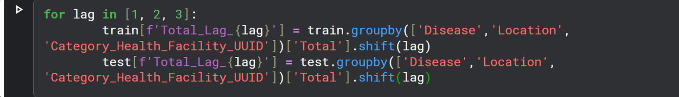
Lag Features
To pick up temporal dependencies, I generated lag features from the target variable (Total). These were grouped by ['Disease','Location', 'Category_Health_Facility_UUID'] and shifted backward by several months. This gave the model a way to “remember” what happened before.
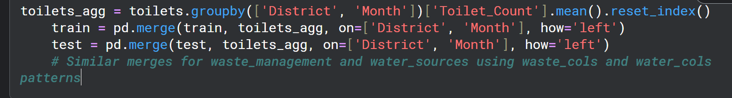
Environmental Data Integration
This part was key. I merged in external variables—soil moisture, surface temps, runoff, humidity, evaporation, and more ('tl2', 'tp', 'swvl1'...). I also brought in data from sanitation sources (toilets, waste, and water infrastructure) and aggregated those by location and month. These variables helped model disease risk based on environmental conditions.
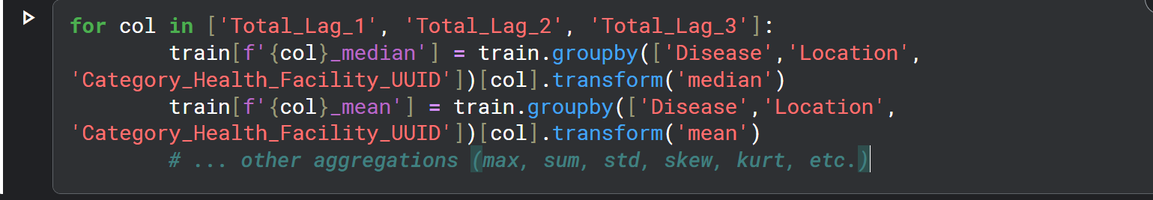
Static Features
From the lagged target variables, I calculated summary stats: mean, median, max, min, skewness, kurtosis, quantiles, etc. Again, all grouped by ['Disease','Location', 'Category_Health_Facility_UUID']. These gave a kind of “profile” of how each disease behaves over time in each location.
🔍 2. Validation Strategy
To avoid overfitting and ensure my models generalized well, I used two main strategies:
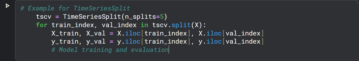
- KFold Cross-Validation – Useful for general robustness and sanity checks.
- TimeSeriesSplit – Especially important for this task. You always want your training data to come before your validation data in a forecasting problem. This simulates real-world deployment conditions.
🧠 3. Modeling Approach
The modeling setup was modular and disease-specific. Here's how I structured it.
Grouping
Every model was trained within groups defined by ['Disease','Location', 'Category_Health_Facility_UUID']. The target was always the Total cases.
Models Used
- LightGBM Regressor – Fast, efficient, and handles large tabular data really well.
- LinearSVR – Solid for capturing linear trends and giving a strong baseline.
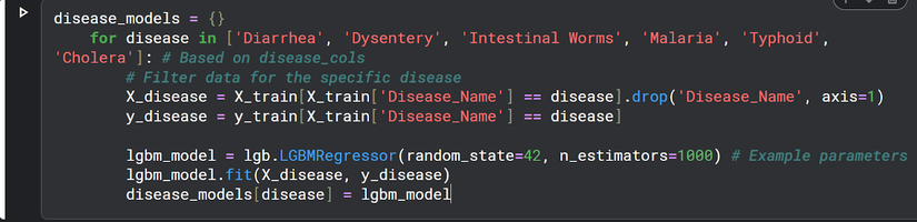
Disease-Specific Training
I trained individual models for each disease: 'Diarrhea', 'Dysentery', 'Intestinal Worms', 'Malaria', 'Typhoid', 'Cholera'. This allowed each model to specialize and learn the nuances of its disease.
Target Transformations
To capture different signals, I trained models on:
- Raw total case values
- Differences from previous months
- Rolling medians
This gave more flexibility to capture both trends and volatility.
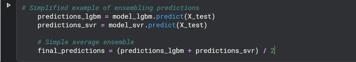
Ensembling
Final predictions came from blending outputs of the different models. LightGBM + LinearSVR + multiple transformations = a more stable and accurate forecast. This helped balance out the strengths and weaknesses of each approach.
✨ Final Thoughts
This challenge really reinforced how critical good feature engineering is—especially when dealing with time-series and environmental data. Having a solid validation pipeline and treating each disease as its own mini-problem also paid off.
Combining multiple models trained on carefully engineered features gave the final edge. It wasn’t just about using fancy models; it was about structuring the problem right, aligning everything with the nature of the data, and being thoughtful in how information flowed from raw input to final prediction.
About Me
I'm Yisak Bule, a Machine Learning Engineer focused on practical, data-driven solutions that tackle real-world problems. I specialize in tabular and time-series modeling and have been fortunate to win multiple Zindi challenges, including this one, the African Credit Scoring Challenge, and the Zindi New User Engagement Prediction Challenge.
My goal is to keep pushing for models that not only perform well on paper but also bring real-world impact.
Thank you @Yisakberhanu for sharing your winning solution. Your solution is really loaded! Big ups and win more!
Thank you for sharing. I see so many others that do not share their solutions and therefore we do not get to learn from them.
I have kind of a stupid question, but how did you know to treat this problem like a time series? I know that there is a time component in the training data but I thought that you could treat it like a regression task and still get decent results. The starter notebook also had such an approach, using RandomForestRegressor.