Have you wondered how data about an object or area can be collected from a distance without any direct contact? Well, you are not alone, if you did.

I am Chigozie Nkwocha, with backgrounds in biochemistry and bioengineering. I snatched my first (hopefully of many) first place wins in the GEOAI Challenge for Cropland Mapping in Dry Environments Challenge.

Follow along in my GitHub repo.

In the field of geography, environmental science and urban planning, remote sensing has been applied to monitor physical events on the Earth’s surface, atmosphere and water bodies using satellite or sensors (aerial or ground-level). These technologies have helped us to track changes in land land use over time, assess damage from natural disasters, and analyse climatic/weather patterns. In agriculture, remote sensing is applied to monitor crop health, soil moisture, and land cover for optimising farming practices. This challenge was a classical example of remote sensing’s application in agriculture.

As we all know, machine learning techniques have opened up a new chapter in how computational techniques can be used to predict an outcome. In this challenge, we were tasked to develop an accurate and cost-effective machine learning to distinguish croplands and non-croplands. However, the focus area was in dry regions: Fergana in Uzbekistan and Orenburg in Russia. These arid and semi-arid regions are characterised by complex agricultural landscapes. For example, they have medium to low vegetation due to minimal precipitation and high evaporation rates causing ground water scarcity, and hence, affecting agriculture in those areas.

Approach

You may be asking: What datasets did I use? What features did I generate and what model(s) did I use? We will get into that in a second.

Datasets

Satellite and sensors pick up physical phenomena and like I mentioned, dry regions have very complex climatic/weather patterns. Based on this, I used three different dataset types. One is the satellite data (Sentinels 1 and 2), climatic data (temperature, precipitation, land surface temperature and evapotranspiration) and the physical structure data (elevation and slope).

Engineered Features

The next step was to preprocess the data and generate relevant features. For this, varying features were generated from the datasets. These features included polarisation ratio, vegetative, water moisture, and bare-soil indices, from the sentinel datasets and water stress index (WSI) from the evapotranspiration data. These features capture vegetation and water availability of these regions.

The next step was to aggregate them into a summary for each reference site in these regions. You may ask why. However, these summaries were aimed to capture the following:

• Temporal dynamics such as growth cycles and seasonal changes.
• Spatial structure by considering proximity to other croplands and regional patterns.
• Rate of change and volatility to identify abrupt transitions and sustained trends.
• Environmental characteristics of these sites by capturing variability, volatility and extremes of these climate and vegetation indices, including the vegetation moisture stress and soil exposure of croplands located in semi-arid regions.

The next lines are a summary (and code snippets) of these engineered features and broad reasons why they were generated.

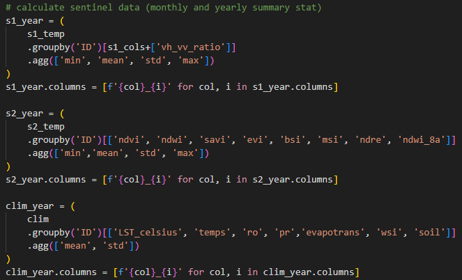
Annual Aggregates

These include, min, max, mean, and standard deviation. They capture long-term trends and variability in vegetation indices, polarization channels and climate variables. Croplands tend to show higher seasonal variability and distinct patterns compared to non-croplands due to planting activities.

# calculate sentinel data (monthly and yearly summary stat)

s1_year = s1_temp.groupby('ID')[s1_cols+['vh_vv_ratio']].agg(

['min', 'mean', 'std', 'max'])

s1_year.columns = [f'{col}_{i}' for col, i in s1_year.columns]

s2_year = s2_temp.groupby('ID')[['ndvi', 'ndwi', 'savi', 'evi',

'bsi', 'msi', 'ndre', 'ndwi_8a']].agg(

['min','mean', 'std', 'max'])

s2_year.columns = [f'{col}_{i}' for col, i in s2_year.columns]

clim_year = clim.groupby('ID')[['LST_celsius', 'temps', 'ro', 'pr',

'evapotrans', 'wsi', 'soil']].agg(['mean', 'std'])

clim_year.columns = [f'{col}_{i}' for col, i in clim_year.columns]

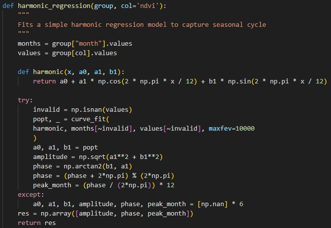
Phenology statistics

These include the peak time and magnitude of periodic patterns. They capture seasonal growth cycles of croplands and non-croplands as croplands tend to show predictable planting and harveting cycles unlike in non-croplands which often lack such pronounced cycles or different timing. A simple harmonic regression was fit.

def harmonic_regression(group, col='ndvi'):

"""

Fits a simple harmonic regression model to capture seasonal cycle

"""

months = group["month"].values

values = group[col].values

def harmonic(x, a0, a1, b1):

return a0 + a1 * np.cos(2 * np.pi * x / 12) + b1 * np.sin(2 * np.pi * x / 12)

try:

invalid = np.isnan(values)

popt, _ = curve_fit(

harmonic, months[~invalid], values[~invalid], maxfev=10000

)

a0, a1, b1 = popt

amplitude = np.sqrt(a1**2 + b1**2)

phase = np.arctan2(b1, a1)

phase = (phase + 2*np.pi) % (2*np.pi)

peak_month = (phase / (2*np.pi)) * 12

except:

a0, a1, b1, amplitude, phase, peak_month = [np.nan] * 6

res = np.array([amplitude, phase, peak_month])

return res

Rate of change per month and acceleration

They quantify how quickly vegetation, bare soil, soil moisture or climate variables change over time and to detect abrupt transitions of these changes over time. Croplands undergo rapid changes during sowing and harvesting periods while non-croplands tend to not have pronounced phenomena. A linear regression model was fit.

def linear_regression(group, ind_col=None, col='ndvi', **kwargs):

"""

Fit a simple linear regression model to capture seasonal cycle:

y = a0 + a1*t

Returns coefficients (a0, a1, b1)

:param group: Grouped data for each ID

:param ind_col: An independent variable

:param col: Dependent variable

:param **kwargs: Keyword arguments.

Accepted arguments include add_diff, add_pct, add_rolling,

n_roll and roll_func

:returns coefficients for each input variable and intercept

"""

add_diff = kwargs.get('add_diff', False)

add_pct = kwargs.get('add_pct', False)

add_rolling = kwargs.get('add_rolling', False)

n_roll = kwargs.get('n_roll', 1)

roll_func = kwargs.get('roll_func', 'mean')

if add_diff and add_pct:

raise Exception('One of add_diff of add_pct must be provided')

if add_diff:

values = group[col].diff()

elif add_pct:

values = group[col].pct_change(fill_method=None).replace(

[np.inf, -np.inf], np.nan)

else:

values = group[col]

if add_rolling: # rolling summary

values = values.rolling(n_roll).agg(roll_func)

if ind_col is None:

X = np.column_stack([np.ones(len(values)), np.arange(len(values))])

else:

X = np.column_stack([np.ones(len(values)), group[ind_col]])

add_seasonal = kwargs.get('add_seasonal', False)

if add_seasonal:

seasons = group['month'].map(encode_season)

X_seasonal, _ = one_hot_encode(seasons)

X = np.c_[X, X_seasonal][:, 1:] # fit regression without intercept

missing = np.isnan(values)

coeffs, _, _, _ = np.linalg.lstsq(X[~missing], values[~missing], rcond=None)

return coeffs

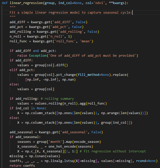
Rolling statistics

We calculated 6-month rolling sum, mean or volatility (standard deviation). These smooth short-term fluctuations and capture medium-term trends and help to identify sustained growth or decline phases, which are common in crop cycles but less so in non-croplands like pastures or steppes.

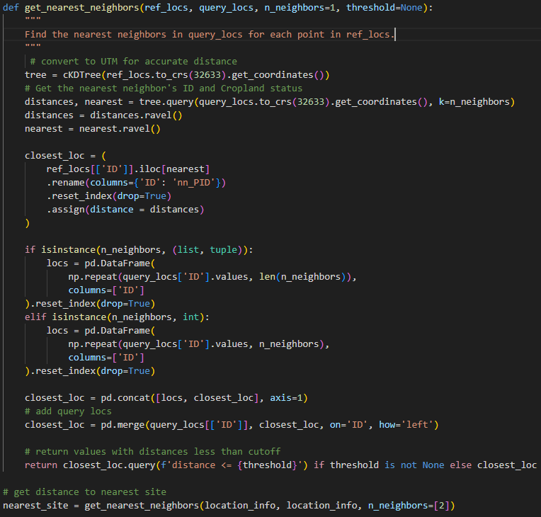
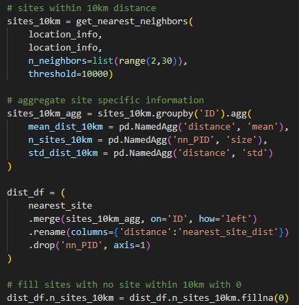
Distance-based features

These include the distance to the nearest site. Others are the average distance, dispersion of sites and the number of sites located within a 10km distance from a reference site. Croplands tend to cluster together and the proximity to other croplands increases the likelihood of a site being used for agricultural purposes.

def get_nearest_neighbors(ref_locs, query_locs, n_neighbors=1, threshold=None):

"""

Find the nearest neighbors in query_locs for each point in ref_locs.

:param ref_locs: Reference location

:param query_locs: Query locations (coordinates)

:param n_neighbours: Int or List: Number of nearest neighbours to return.

If int, nearest neighbours up to set value is returned. if list,

only nearest neighbours in the list are returned

:param threshold: Distance threshold to return (Distance in metres)

"""

# convert to UTM for accurate distance

tree = cKDTree(ref_locs.to_crs(32633).get_coordinates())

# Get the nearest neighbor's ID and Cropland status

distances, nearest = tree.query(

query_locs.to_crs(32633).get_coordinates(),

k=n_neighbors)

distances = distances.ravel()

nearest = nearest.ravel()

closest_loc = (

ref_locs[['ID']].iloc[nearest]

.rename(columns={'ID': 'nn_PID'})

.reset_index(drop=True)

.assign(distance = distances)

)

if isinstance(n_neighbors, (list, tuple)):

locs = pd.DataFrame(np.repeat(

query_locs['ID'].values,

len(n_neighbors)),

columns=['ID']).reset_index(drop=True)

elif isinstance(n_neighbors, int):

locs = pd.DataFrame(np.repeat(

query_locs['ID'].values,

n_neighbors),

columns=['ID']).reset_index(drop=True)

closest_loc = pd.concat([locs, closest_loc], axis=1)

# add query locs

closest_loc = pd.merge(

query_locs[['ID']], closest_loc,

on='ID', how='left')

# return values with distances less than cutoff

return closest_loc.query(

f'distance <= {threshold}'

) if threshold is not None else closest_loc

# get distance to nearest site

nearest_site = get_nearest_neighbors(location_info, location_info, n_neighbors=[2])

# sites within 10km distance

sites_10km = get_nearest_neighbors(

location_info,

location_info,

n_neighbors=list(range(2,30)),

threshold=10000)

# aggregate site specific information

sites_10km_agg = sites_10km.groupby('ID').agg(

mean_dist_10km = pd.NamedAgg('distance', 'mean'),

n_sites_10km = pd.NamedAgg('nn_PID', 'size'),

std_dist_10km = pd.NamedAgg('distance', 'std')

)

dist_df = (nearest_site

.merge(sites_10km_agg, on='ID', how='left')

.rename(columns={'distance':'nearest_site_dist'})

.drop('nn_PID', axis=1)

)

# fill sites with no site within 10km with 0

dist_df.n_sites_10km = dist_df.n_sites_10km.fillna(0)

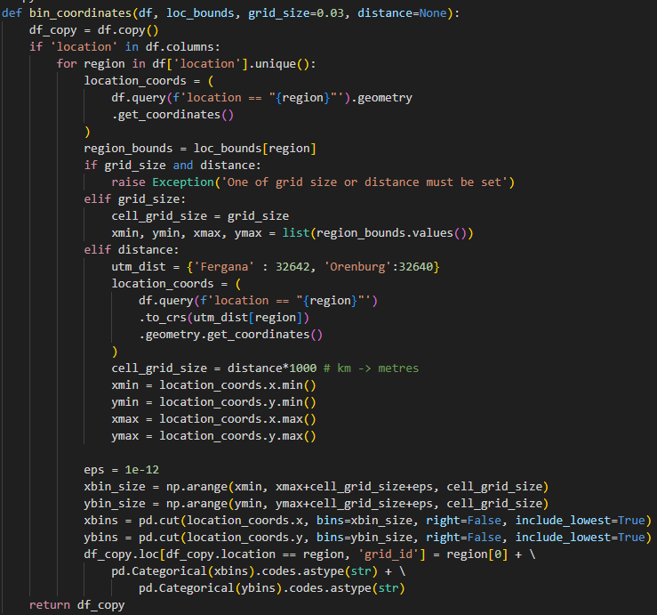
Grid-based aggregation

This captures regional vegetative or climate patterns of sites located within a region/area. The function below was used to bin coordinates into grids.

def bin_coordinates(df, loc_bounds, grid_size=0.03, distance=None):

df_copy = df.copy()

if 'location' in df.columns:

for region in df['location'].unique():

location_coords = df.query(

f'location == "{region}"').geometry.get_coordinates()

region_bounds = loc_bounds[region]

if grid_size and distance:

raise Exception('One of grid size or distance must be set')

elif grid_size:

cell_grid_size = grid_size

xmin, ymin, xmax, ymax = list(region_bounds.values())

elif distance:

utm_dist = {'Fergana' : 32642, 'Orenburg':32640}

location_coords = (

df

.query(f'location == "{region}"')

.to_crs(utm_dist[region])

.geometry.get_coordinates()

)

cell_grid_size = distance*1000 # km -> metres

xmin = location_coords.x.min()

ymin = location_coords.y.min()

xmax = location_coords.x.max()

ymax = location_coords.y.max()

eps = 1e-12

xbin_size = np.arange(xmin, xmax+cell_grid_size+eps, cell_grid_size)

ybin_size = np.arange(ymin, ymax+cell_grid_size+eps, cell_grid_size)

xbins = pd.cut(location_coords.x, bins=xbin_size,

right=False, include_lowest=True)

ybins = pd.cut(location_coords.y, bins=ybin_size,

right=False, include_lowest=True)

df_copy.loc[df_copy.location == region, 'grid_id'] = region[0] + \

pd.Categorical(xbins).codes.astype(str) + \

pd.Categorical(ybins).codes.astype(str)

return df_copy

Clustering

Site coordinates for each region: Fergana and Orenburg were clustered into four groups (optimal number of clusters selected from elbow method).

These engineered features were then saved and used for modelling.

Modelling and feature importance

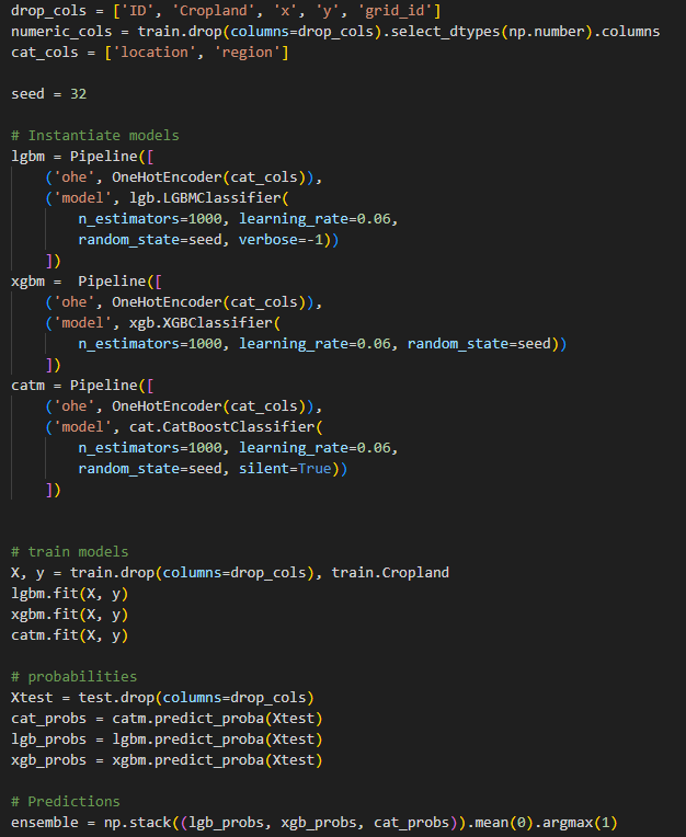
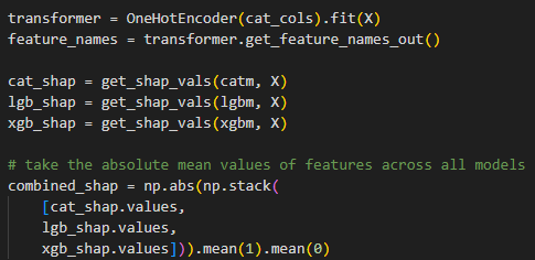
Now, with all features generated and saved, the next step was to develop a machine learning model to classify croplands and non-croplands. Three gradient boosting models: catboost, lightgbm and xgboost were used. Irrelevant features were dropped and one-hot encoding was applied to categorical featues (region and cluster groups). The final model was obtained 7 by averaging the probabilities of each model and assigning a cropland class to probabilities above 0.5 and non-cropland class, otherwise.

You may wondering if I did not use a train-test split method to evaluate performance on a held out data before submitting on the leaderboard. Well, I did that at first, and was getting a good score. So, I decided to fit a final model on all the training data and then make predictions on the test data. From a 5-fold cross-validation approach, all three models had about 0.87+ in accuracy, which mirrors the private leaderboard score of about 0.85.

drop_cols = ['ID', 'Cropland', 'x', 'y', 'grid_id']

numeric_cols = train.drop(columns=drop_cols).select_dtypes(np.number).columns

cat_cols = ['location', 'region']

seed = 32

# Instantiate models

lgbm = Pipeline([

('ohe', OneHotEncoder(cat_cols)),

('model', lgb.LGBMClassifier(

n_estimators=1000, learning_rate=0.06,

random_state=seed, verbose=-1))

])

xgbm = Pipeline([

('ohe', OneHotEncoder(cat_cols)),

('model', xgb.XGBClassifier(

n_estimators=1000, learning_rate=0.06, random_state=seed))

])

catm = Pipeline([

('ohe', OneHotEncoder(cat_cols)),

('model', cat.CatBoostClassifier(

n_estimators=1000, learning_rate=0.06,

random_state=seed, silent=True))

])

# train models

X, y = train.drop(columns=drop_cols), train.Cropland

lgbm.fit(X, y)

xgbm.fit(X, y)

catm.fit(X, y)

# probabilities

Xtest = test.drop(columns=drop_cols)

cat_probs = catm.predict_proba(Xtest)

lgb_probs = lgbm.predict_proba(Xtest)

xgb_probs = xgbm.predict_proba(Xtest)

# Predictions

ensemble = np.stack((lgb_probs, xgb_probs, cat_probs)).mean(0).argmax(1)

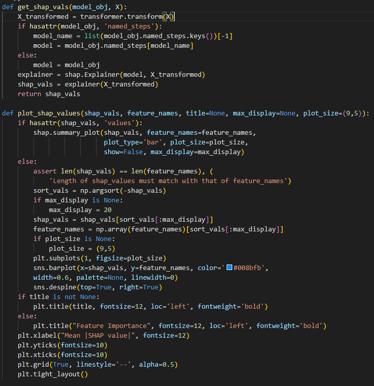
What are the important features?

It doesn't stop at developing a model, we need to understand the features that enabled these models to arrive at their predictions. To accomplish this, I computed and averaged the absolute shap values for each feature for each model. It was discovered that for the three models, the top features were mostly from the sentinel datasets. These include the polarisation channels (VV and VH), vegetative indices, bare soil indices (BSI) and moisture stress index (MSI). These features are characteristic to arid and semi-arid regions.

To get a consensus score for features in the three models, we averaged these shap values. Here, we see that the peak time, represented by phase, annual minimum or maximum values, and annual deviations, the magnitude of their periodic patterns, represented by the amplitude, are some features that distinguish croplands from non-croplands. Others include their rate of change (or percentage change) per month, the rate of change of monthly changes, (known as the acceleration), the variability of these changes (standard deviation), slope of the site, and the distance to the closest site.

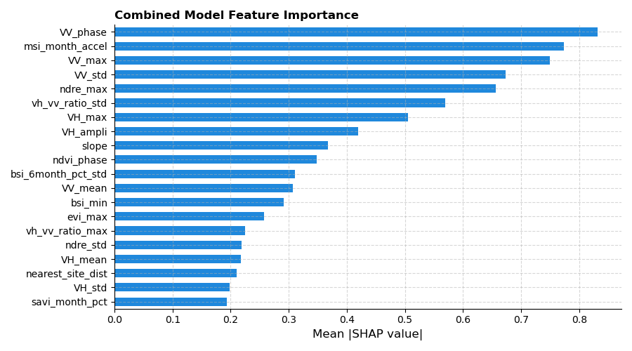
Figure 1: Combined Feature Importance

def get_shap_vals(model_obj, X):

X_transformed = transformer.transform(X)

if hasattr(model_obj, 'named_steps'):

model_name = list(model_obj.named_steps.keys())[-1]

model = model_obj.named_steps[model_name]

else:

model = model_obj

explainer = shap.Explainer(model, X_transformed)

shap_vals = explainer(X_transformed)

return shap_vals

def plot_shap_values(shap_vals, feature_names, title=None,

max_display=None, plot_size=(9,5)):

if hasattr(shap_vals, 'values'):

shap.summary_plot(shap_vals, feature_names=feature_names,

plot_type='bar', plot_size=plot_size,

show=False, max_display=max_display)

else:

assert len(shap_vals) == len(feature_names), (

'Length of shap_values must match with that of feature_names')

sort_vals = np.argsort(-shap_vals)

if max_display is None:

max_display = 20

shap_vals = shap_vals[sort_vals[:max_display]]

feature_names = np.array(feature_names)[sort_vals[:max_display]]

if plot_size is None:

plot_size = (9,5)

plt.subplots(1, figsize=plot_size)

sns.barplot(x=shap_vals, y=feature_names, color='#008bfb',

width=0.6, palette=None, linewidth=0)

sns.despine(top=True, right=True)

if title is not None:

plt.title(title, fontsize=12, loc='left', fontweight='bold')

else:

plt.title("Feature Importance", fontsize=12, loc='left', fontweight='bold')

plt.xlabel("Mean |SHAP value|", fontsize=12)

plt.yticks(fontsize=10)

plt.xticks(fontsize=10)

plt.grid(True, linestyle='--', alpha=0.5)

plt.tight_layout()

transformer = OneHotEncoder(cat_cols).fit(X)

feature_names = transformer.get_feature_names_out()

cat_shap = get_shap_vals(catm, X)

lgb_shap = get_shap_vals(lgbm, X)

xgb_shap = get_shap_vals(xgbm, X)

# take the absolute mean values of features across all models

combined_shap = np.abs(np.stack(

[cat_shap.values,

lgb_shap.values,

xgb_shap.values])).mean(1).mean(0)

Final Thoughts

From this challenge, we learned how machine learning can accurately distinguish croplands and non-croplands using remote sensing data. We also see that generating rich and relevant features related to the climatic patterns and physical characteristics of the region of interest, as well as, their spatial information, are important to achieving this. Similarly, this solution offers a cheap and efficient method to adapt to other regions without the need to physically visit these sites.

For more on the datasets and Python scripts, here is a link to the repository.

About Me

I am Chigozie Nkwocha, with backgrounds in biochemistry and bioengineering. I am a data scientist, and would-be machine learning engineer, with a passion for developing practical solutions to real-world problems. With strong skills in R, SQL and Python, I have applied data science and machine learning techniques in health, biology, environment, and business. I specialise mostly in tabular data but gradually transitioning into unstructured datasets.

I have participated in many competitions here on Zindi, and still participating. Participating here on Zindi has helped me gain experience in various fields and has honed (and still honing) my skill sets.