There has been an increase in deep learning applications in recent years, such as credit card fraud detection in finance, smart farming in agriculture, and others.

In this tutorial, we will be creating a simple crop disease detection using PyTorch. We will use a plant leaf dataset that consists of 39 different classes of crop diseases with RGB images. We will leverage the power of the Convolutional Neural Network (CNN) to achieve this.

Prerequisites

• Install PyTorch
• Basic Understanding on Neural Networks in this case Convolutional Neural Network (CNN)

1. Install PyTorch

Follow the guidelines on the website to install PyTorch. Based on your operating system, the package, and the programming language, you get the command to run to install.

2. Understanding of Convolutional Neural Network (CNN)

CNN is a type of neural network which includes convolutional and pooling layers.

• Convolutional layer - contains a set of filters whose height and weight are smaller than the input image. These weights are then trained.
• Pooling layer - Incorporated between two convolutional layers, a pooling layer reduces the number of parameters and computation power by down-sampling the images through an activation function.
• Fully connected layer - Takes the convolutional and pooling layer results, processes and reaches a classification decision.

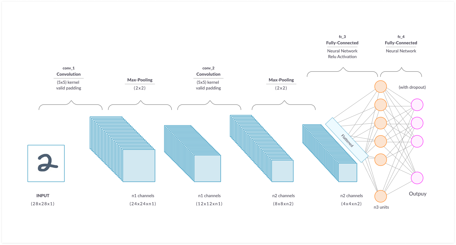
Creating a CNN will involve the following:

Step 1: Data loading and transformation

Step 2: Defining the CNN architecture

Step 3: Define loss and optimizer functions

Step 4: Training the model using the training set of data

Step 5: Validating the model using the test set

Step 6: Predict

• We will tackle this tutorial in a different format, where I will show the standard errors I encountered while starting to learn PyTorch.

Step 1: Data loading and transformation

1.1 import our packages

import torch 

from torchvision import datasets, transforms, models

1.2 Load data

Set up the data directory folder

data_dir = "data/"

Every image is in the form of pixels that translate into arrays. PyTorch uses PIL - A python library for image processing.

Pytorch uses the torchvision module to load datasets. The torchvision package consists of popular datasets, model architectures, and common image transformations for computer vision. We will use the ImageFolder class to load our dataset.

To load data using the ImageFolder data must be arranged in this format:

    root/dog/xxx.png

    root/dog/xxy.png

    root/dog/xxz.png

    root/cat/123.png

    root/cat/nsdf3.png

    root/cat/asd932_.png

and NOT this format:

    root/xxx.png

    root/xxy.png

    root/123.png

    root/nsdf3.png

1.3 Split the dataset into train and validation sets

It’s advisable to set aside validation data for inference purposes.

I have created a module split_data that splits any given image classification data into train and validation with a ratio of 80:20.

train_data = datasets.ImageFolder(data_dir + '/train')

val_data = datasets.ImageFolder(data_dir + '/val')

1.4 Make the data Iterable

dataiter = iter(train_data)

images, clases = dataiter

print(type(images))

The command above raises:

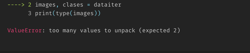
This means we can not iterate (meaning loop through) over the dataset. Pytorch use DataLoader to make the dataset iterable.

train_loader = torch.utils.data.DataLoader(train_data, shuffle=True)

val_loader = torch.utils.data.DataLoader(val_data,)

_________________

dataiter = iter(train_loader)

images, clases = dataiter.next()

print(type(images))

The code above raises:

The get item method of ImageFolder returns an unprocessed PIL image. PyTorch uses tensors; since we will pass this data through PyTorch models, we need to transform the image to a tensor before using the data loader.

train_transforms = transforms.Compose([transforms.ToTensor()])

val_transforms = transforms.Compose([transforms.ToTensor(),])

train_data = datasets.ImageFolder(data_dir + '/train', transform=train_transforms)

val_data = datasets.ImageFolder(data_dir + '/val', transform=val_transforms)

train_loader = torch.utils.data.DataLoader(train_data, batch_size=8, shuffle=True)

val_loader = torch.utils.data.DataLoader(val_data, batch_size=8)

batch_size means run eight samples per iterations.

Rerun the dataiter. Which will raise a runtime error;

In most scenarios, you will get images that are of different dimensions. In image processing, it’s recommended to transform the images to equal dimensions to ensure that the model can not prioritize predicting based on the dimensions. Thus we need to resize the images to the same shape then transform it into a tensor. The code below which combines all the steps we have discussed above.

Data Transformation and Augmentation

train_transforms = transforms.Compose([transforms.RandomRotation(30), #data augumnetation

                                       transforms.RandomResizedCrop(224),#resize

                                       transforms.RandomHorizontalFlip(), #data augumnetation

                                       transforms.ToTensor()])

val_transforms = transforms.Compose([transforms.RandomResizedCrop(224), #resize

                                      transforms.ToTensor()])

train_data = datasets.ImageFolder(data_dir + '/train', transform=train_transforms)

val_data = datasets.ImageFolder(data_dir + '/val', transform=val_transforms)

train_loader = torch.utils.data.DataLoader(train_data, batch_size=8, shuffle=True)

val_loader = torch.utils.data.DataLoader(val_data, batch_size=8)

dataiter = iter(train_loader)

images, classes = dataiter.next()

print(type(images))

print(images.shape)

print(classes.shape)

Step 2: Model architecture

We’ll be using PyTorch NN module to build models.

When creating CNN, understanding the output dimensions after every convolutional and pooling layer is important.

2.1 Calculate output dimensions

Below is the formula to calculate dimensions through a convolutional layer

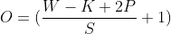
Where;

O - The output height/width

W - The input height/width

K - The kernel size

P - Padding

S - Stride

The formula below calculates dimensions after a max pool layer

We will create a sample CNN model of this architecture:

• 2 convolutional layers
• 2 max-pooling layers
• 1 fully connected layer

Input_image shape(RGB) = 224, 224, 3

1st convolutional layer

• W = 224
• K = 3
• P = 0
• S = 1

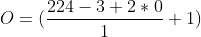
(224 - 3 ) + 1 = 222

the output will be 222 x 222 x 16 : Note 16 in the channel/color dimensions we have selected.

1st max-pooling layer

shape = 222 x 222 x 16 k = 2

222 / 2 = 111

The output image will be 111 x 111 x 16 (the color channel does not change after a max pool layer)

2nd Convolutional Layer

• W = 111
• K = 3
• P = 1
• S = 2

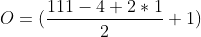
(111 - 3 + 2*1)/2 + 1 = 56

output image 56x 56 x 32

2nd max-pooling layer

56/2 = 28

output image 28 x 28 x 32

Fully connected layer

In the fully connected layer, you pass a flattened image, and the number of output classes required in this case is 39.

import torch.nn as nn

import numpy as np

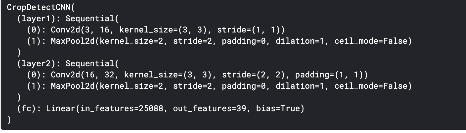
class CropDetectCNN(nn.Module):

    # initialize the class and the parameters

    def __init__(self):

        super(CropDetectCNN, self).__init__()

        # convolutional layer 1 & max pool layer 1

        self.layer1 = nn.Sequential(

            nn.Conv2d(3, 16, kernel_size=3),

            nn.MaxPool2d(kernel_size=2))

        # convolutional layer 2 & max pool layer 2

        self.layer2 = nn.Sequential(

            nn.Conv2d(16, 32, kernel_size=3, padding=1, stride=2),

            nn.MaxPool2d(kernel_size=2))

        #Fully connected layer

        self.fc = nn.Linear(32*28*28, 39)

    # Feed forward the network

    def forward(self, x):

        out = self.layer1(x)

        out = self.layer2(out)

        out = out.reshape(out.size(0), -1)

        out = self.fc(out)

        return out

model = CropDetectCNN()

print(model)

Step 3: Loss and Optimizer

Loss determines how far the model deviates from predicting true values. Optimizer is the function used to change the neural networks’ attributes/parameters such as weights and learning rates.

These functions are dependant on the type of machine learning problem you are trying to solve. In our case, we are dealing with multi-class classification. You can research more on loss and optimization in neural networks.

For this case, we’ll use Cross-Entropy Loss and Stochastic Gradient Descent(SGD)

import torch.optim as optim

criterion = nn.CrossEntropyLoss()

optimizer = optim.SGD(model.parameters(), lr=0.01)

Image analysis requires very high processing power, you can leverage free GPUs in the market. PyTorch uses CUDA to enable developers to run their products on GPU enabled environment.

# run on GPU if available else run on a CPU

device = torch.device("cuda" if torch.cuda.is_available() else "cpu")

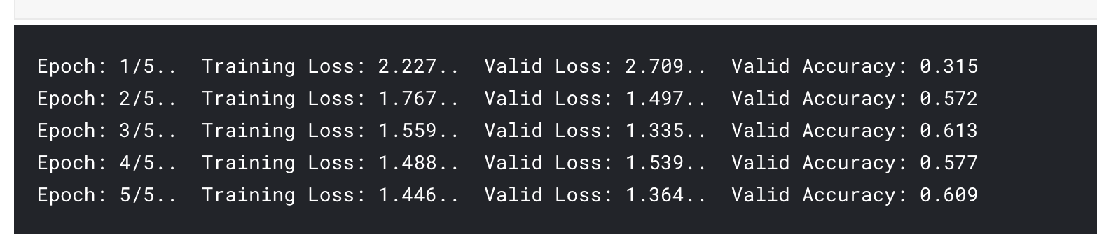
Step 4 & 5: Model Training and Validation

epochs = 1 # run more iterations

for epoch in range(epochs):

    running_loss = 0

    for images, classes in train_loader:

        # To device - to transfrom the image and classes to CPU|GPU

        images, classes = images.to(device), classes.to(device)

        # clears old gradients from the last step

        optimizer.zero_grad()

        # train the images

        outputs = model(images)

        #calculate the loss given the outputs and the classes

        loss = criterion(outputs, classes)

        # compute the loss of every parameter

        loss.backward()

        # apply the optimizer and its parameters

        optimizer.step()

        #update the loss

        running_loss += loss.item()

    else:

        validation_loss = 0

        accuracy = 0

        # to make the model run faster we are using the gradients on the train

        with torch.no_grad():

            # specify that this is validation and not training

            model.eval()

            for images, classes in val_loader:          

                # Use GPU

                images, classes = images.to(device), classes.to(device)

                # validate the images

                outputs = model(images)

                # compute validation loss

                loss = criterion(outputs, classes)

                #update loss

                validation_loss += loss.item()

                # get the exponential of the outputs

                ps = torch.exp(outputs)

                #Returns the k largest elements of the given input tensor along a given dimension.

                top_p, top_class = ps.topk(1, dim=1)

                # reshape the tensor

                equals = top_class == classes.view(*top_class.shape)

                # calculate the accuracy.

                accuracy += torch.mean(equals.type(torch.FloatTensor))

        # change the mode to train for the next epochs

        model.train()

        print("Epoch: {}/{}.. ".format(epoch+1, epochs),

              "Training Loss: {:.3f}.. ".format(running_loss/len(train_loader)),

              "Valid Loss: {:.3f}.. ".format(validation_loss/len(val_loader)),

              "Valid Accuracy: {:.3f}".format(accuracy/len(val_loader)))

Step 6: Model prediction

Let’s see how our model can predict one of the images.

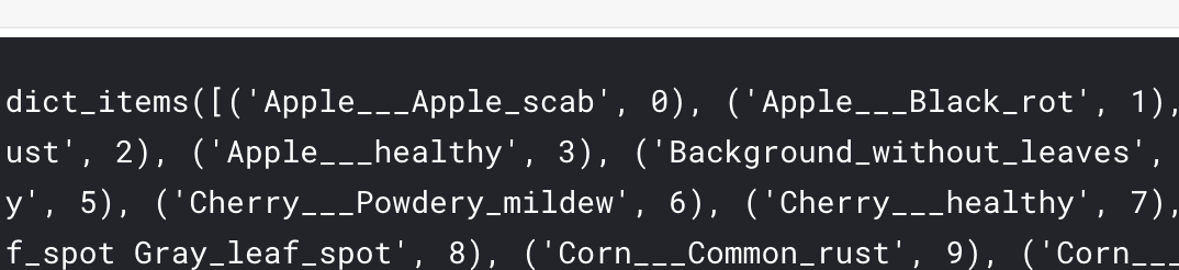
In the PyTorch ImageFolder we used, we have a variable class_to_idx which converted the class names to respective index. Since training uses the index we need to convert the predicted index to the corresponding class name

model.class_to_idx = train_data.class_to_idx

model.class_to_idx.items()

6.1 Process the image

• We need to transform the image into the desired shape and to a tensor before predicting it.

from PIL import Image

import numpy as np

# Plot the image

def imshow(image_numpy_array):

    fig, ax = plt.subplots()

    # convert the shape from (3, 256, 256) to (256, 256, 3)

    image = image.transpose(0, 1, 2)

    ax.imshow(image)

    ax.set_xticklabels('')

    ax.set_yticklabels('')

    return ax

def process_image(image_path):

    test_transform = transforms.Compose([transforms.RandomResizedCrop(224),

                                         transforms.ToTensor()])

    im = Image.open(image_path)

    imshow(np.array(im))

    im = test_transform(im)

    return im

• Pass the image through the already trained model.

def predict(image, model):

    # we have to process the image as we did while training the others

    image = process_image(image)

    #returns a new tensor with a given dimension

    image_input = image.unsqueeze(0)

    # Convert the image to either gpu|cpu

    image_input.to(device)

    # Pass the image through the model

    outputs = model(image_input)

    ps = torch.exp(outputs)

    # return the top 5 most predicted classes

    top_p, top_cls = ps.topk(5, dim=1)

    # convert to numpy, then to list 

    top_cls = top_cls.detach().numpy().tolist()[0]

    # covert indices to classes

    idx_to_class = {v: k for k, v in model.class_to_idx.items()}

    top_cls = [idx_to_class[top_class] for top_class in top_cls]

    return top_p, top_cls

Visualization

import seaborn as sns

import matplotlib.pyplot as plt

def plot_solution(image_path, ps, classes):

    plt.figure(figsize = (6,10))

    image = process_image(image_path)

    plt.subplot(2,1,2)

    sns.barplot(x=ps, y=classes, color=sns.color_palette()[2]);

    plt.show()

Image sample prediction

• The image sample is one of the validation set images. We already know that the plant leaf disease is Apple___Apple_scab. Let’s see how our simple 2 layers CNN predicts.

image = "data/val/Apple___Apple_scab/image (102).JPG"

ps, classes = predict(image, model)

ps = ps.detach().numpy().tolist()[0]

print(ps)

print(classes)

plot_solution(image, ps, classes)

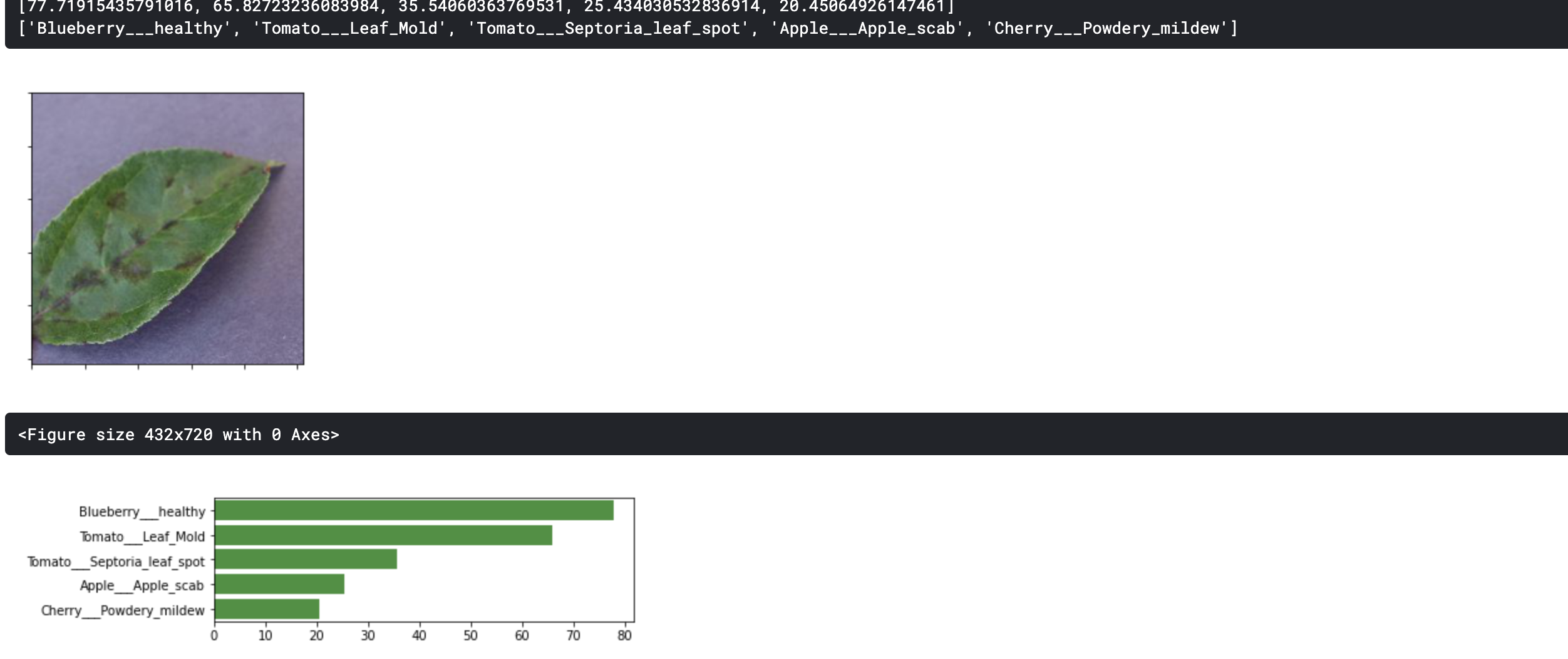
• Our sample model is not able to correctly differentiate between different plant leaves.
• TODOs, try increasing the number of epochs and also create more convolutional layers. Is the prediction better?

Conclusion

• In this tutorial, we developed a simple CNN that should get you started on understanding Neural Network and Image processing with Pytorch.
• The project, however, is build using deep Convolutional Neural Networks of pre-trained densenet 201. This is the concept of transfer learning, which is the improvement of a model in a new project scenario by transferring knowledge from a related project scenario that has already been trained.
• Below is the output from the transfer learning project on the same image.

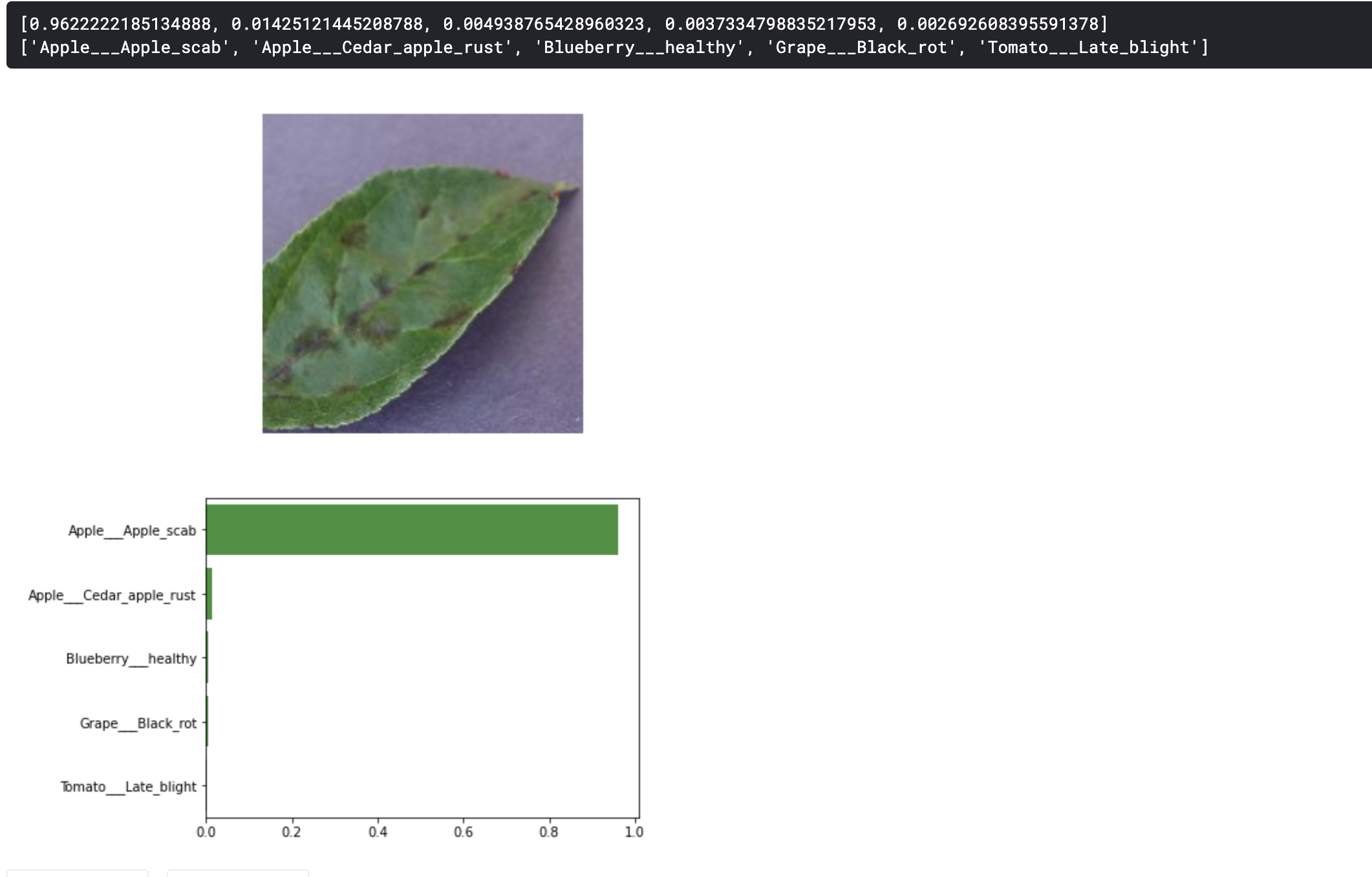
• We can see that our pre-trained model was able to make a better prediction than our simple CNN. We’ll learn about transfer learning in part 2 of the tutorial.

About the author:

Rose Wambui is an experienced Software Engineer with a demonstrated history of working in the information technology and services industry. She is skilled in data visualization, data analysis, data engineering, machine learning, and software development. Rose is a strong engineering professional with a Bsc. computer forensics and security, focused in IT security from Jaramogi Oginga Odinga University of Science and Technology, and currently works as a Zindi data scientist.