Using a text classifier to predict various categories in Malawi News articles using SMOTE and SGDClassifier.

Introduction

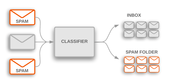
Text classification is common among the applications we use on a daily basis. For example, email providers use text classification to filter out spam emails from your inbox. The other most common use of text classification is in customer care, where they use sentiment analysis to differentiate bad reviews from good reviews (ADDI AI 2050). The modern use of text classification has excelled to more advanced forms of classification, which include multilanguage and multilabel classification.

In recent years, the English language has come a long way, but training classification models on low resource languages, at varying lengths, still pose difficulties. In this Zindi competition, we are provided with news articles written in the Malawian language, Chichewa, and we train our model on multi-label classification as there are 19 categories of news. The texts are made up of news articles of varying lengths, so determining a good model will be a challenging task.

The project code is simple and effective on competitive grounds, and I have experimented with Vectorizer, Porter stemmer for test preprocessing. I have also used multiple methods to clean my text to improve overall model performance. In the end, I decided to use Sklearn Stochastic Gradient Decent (SGD) classifier for predicting news categories. I have also experimented with various neural networks and gradient boosting models, but they all failed as simple logistics regression with minimum hyperparameter tuning works well on this data.

Code

Deepnote environment was used to train the classification model.

Import Libraries

from sklearn.feature_extraction.text import TfidfVectorizer

from sklearn.metrics import accuracy_score, classification_report, confusion_matrix

from sklearn.model_selection import train_test_split

from sklearn.linear_model import SGDClassifier

from sklearn.preprocessing import LabelEncoder

from nltk.stem import WordNetLemmatizer

from imblearn.over_sampling import SMOTE

import matplotlib.pyplot as plt

import seaborn as sns

import pandas as pd

import numpy as np

import re

import warnings

warnings.filterwarnings("ignore")

Import and download the nltk;

import nltk

nltk.download('wordnet')

>>[nltk_data] Downloading package wordnet to /root/nltk_data...
>> [nltk_data]   Package wordnet is already up-to-date!
>> True

Read Train/ Test Dataset

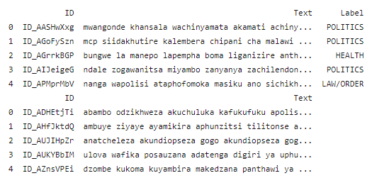
The data was collected from various news publishing companies in Malawi. tNyasa Ltd Data Science Lab has used three main broadcasters: the Nation Online newspaper, Radio Maria, and the Malawi Broadcasting Corporation.

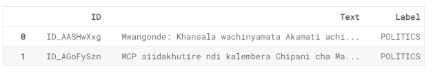
The Training Data contains three columns:

• ID: Unique Identifier
• Text: news articles
• Label: classifications of news articles.

The task is to classify the news articles into one of 19 categories.

As you can see; the train data set has 1436 samples, whereas, the test data set has 620 samples.

train_data = pd.read_csv("../input/malawi-news-classification-challenge/Train.csv")

test_data = pd.read_csv("../input/malawi-news-classification-challenge/Test.csv")

print(train_data.shape)

print(test_data.shape)

>> (1436, 3)

>> (620, 2)

Let’s look at the top two rows;

train_data.head(2)

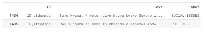
Now let’s look at the bottom two rows;

train_data.tail(2)

Lastly, let’s look at the Train Dataset label distribution.

It is evident that we have unbalanced distribution of classes which can cause problems during machine learning model training. The POLITICS category takes the lead in our train dataset.

train_data.Label.value_counts().plot(kind='bar');

Cleaning Text

• Removing special characters.
• Lowering text.
• Lemmatizing words.

chichewa = ['i', 'ine', 'wanga', 'inenso', 'ife', 'athu', 'athu', 'tokha', 'inu', 'ndinu','iwe ukhoza', 'wako','wekha','nokha','iye','wake','iyemwini','icho','ndi','zake','lokha','iwo','awo','iwowo','chiyani','amene', 'uyu', 'uyo', 'awa', "ndili", 'ndi', 'ali','anali','khalani','akhala','kukhala',' Khalani nawo','wakhala','anali','chitani','amachita','kuchita', 'a', 'an', 'pulogalamu ya', 'ndi', 'koma', 'ngati', 'kapena', 'chifukwa', 'monga', 'mpaka', 'pamene', 'wa', 'pa ',' by','chifukwa' 'ndi','pafupi','kutsutsana','pakati','kupyola','nthawi', 'nthawi','kale','pambuyo','pamwamba', 'pansipa', 'kuti', 'kuchokera', 'mmwamba', 'pansi', 'mu', 'kunja', 'kuyatsa', 'kuchoka', 'kutha', 'kachiwiri', 'kupitilira','kenako',' kamodzi','apa','apo','liti','pati','bwanji','onse','aliyense','onse','aliyense', 'ochepa', 'zambiri', 'ambiri', 'ena', 'otero', 'ayi', 'kapena', 'osati', 'okha', 'eni', 'omwewo', 'kotero',' kuposa','nawonso',' kwambiri','angathe','ndidzatero','basi','musatero', 'musachite',' muyenera', 'muyenera kukhala','tsopano', 'sali', 'sindinathe','​​sanachite','satero','analibe', 'sanatero','sanachite','sindinatero','ayi','si', 'ma', 'sizingatheke','mwina','sayenera', 'osowa','osafunikira', 'shan' , 'nenani', 'sayenera', 'sanali', 'anapambana', 'sangachite', 'sanakonde', 'sangatero']

wn = WordNetLemmatizer()

def text_preprocessing(review):

    review = re.sub('[^a-zA-Z]', ' ', review)

    review = review.lower()

    review = review.split()

    review = [wn.lemmatize(word) for word in review if not word in chichewa]

    review = ' '.join(review)

    return review

Applying the text preprocessing

Simply apply the above function on both test and train datasets.

train_data['Text'] = train_data['Text'].apply(text_preprocessing)

test_data['Text'] = test_data['Text'].apply(text_preprocessing)

print(train_data.head())

print(test_data.head())

View Output

As you can see, we have much cleaner text, which is ready to be trained on our model.

Text Vectorization

Term Frequency Inverse Document Frequency (TFIDF). The algorithm converts text data into a meaningful representation of numbers (Medium). The transformation is necessary as the machine learning model doesn’t understand text data, so we need to convert the data into a numerical format. We will be converting our text data into vectors using Sklearn TFIDF transformation, and our final data shape will have 49 480 columns/features.

vectorizer = TfidfVectorizer()

X = vectorizer.fit_transform(train_data['Text']).toarray()

training = pd.DataFrame(X, columns=vectorizer.get_feature_names())

print(training.shape)

X_test_final = vectorizer.transform(test_data['Text']).toarray()

test_new = pd.DataFrame(X_test_final, columns=vectorizer.get_feature_names())

print(test_new.shape)

>> (1436, 49480)

>> (620, 49480)

Preparing Data for Training

Using our train data to get X (training features) and y (Target). We will use Label encoding to convert string labels into numerical labels such as [1,2,3….]

X = training 

y = train_data['Label']

Label Encoding

label_encoder = LabelEncoder() 

y_label = label_encoder.fit_transform(y)

Our data is quite unbalanced as shown in Figure 1. The Politics category has the highest number of samples, followed by categories; Social and Religion. This imbalance of data will cause our model to perform badly, so to improve model performance, we must balance our data by either removing extra samples or using the Synthetic Minority Over-sampling Technique (SMOTE). SMOTE is an oversampling technique where the synthetic samples are generated for the minority class (analyticsvidhya.com).

In our case, all the minority classes will be synthesized to match the majority class; Politics. As you can see, all of the classes have the same number of samples, which is perfectly balanced.

smote = SMOTE() 

X, y_label = smote.fit_resample(X,y_label)
np.bincount(y_label)

>> array([279, 279, 279, 279, 279, 279, 279, 279, 279, 279, 279, 279, 279, 279, 279, 279, 279, 279, 279, 279])

Training Model

I have used:

• Neural networks
• XGBoost
• LGBM classifiers
• Catboost
• Automl
• Logistic Regression
• Tabnet
• Random Forest Classifier

However, they all failed in comparison to SGD. In short, using SGD classification with simple hyperparameter tuning will give you the best results. This estimator implements regularized linear models with stochastic gradient descent (SGD) learning (sklearn.linear_model.SGDClassifier).

• Splitting into Train and Test: 10% Testing dataset
• Using SGDClassifier: Use loss function as a hinge with alpha=0.0004, max_iter=20

X_train, X_test, y_train, y_test = train_test_split(X, y_label, test_size=0.1, random_state=0)

model = SGDClassifier(loss='hinge', 

                      alpha=4e-4, 

                      max_iter=20, 

                      verbose=False)

model.fit(X_train, y_train)

>> SGDClassifier(alpha=0.0004, max_iter=20, verbose=False)

Evaluation

Our model performed quite well with the oversampling technique.

The training model without SMOTE got the highest accuracy of 55%.

pred = model.predict(X_test)

print("Train Accuracy Score:",round(model.score(X_train, y_train),2))

print("Test Accuracy Score:",round(accuracy_score(y_test, pred),2))

Train Accuracy Score: 0.99

Test Accuracy Score: 0.95

Classification Report

The classification report for every class is also amazing as the majority of the f1-score is between 90 to 100%.

print(classification_report(y_test, pred))

                 precision  recall  f1-score   support

           0       1.00      1.00      1.00        30

           1       1.00      1.00      1.00        25

           2       0.96      0.83      0.89        29

           3       0.92      1.00      0.96        22

           4       0.97      1.00      0.98        29

           5       1.00      1.00      1.00        29

           6       0.87      0.90      0.89        30

           7       0.90      0.93      0.92        30

           8       0.95      1.00      0.98        20

           9       1.00      1.00      1.00        37

          10       1.00      1.00      1.00        25

          11       0.90      0.75      0.82        24

          12       1.00      1.00      1.00        31

          13       0.79      0.92      0.85        25

          14       0.82      0.62      0.71        29

          15       0.95      0.95      0.95        19

          16       1.00      1.00      1.00        30

          17       0.94      1.00      0.97        32

          18       0.91      1.00      0.95        30

          19       1.00      1.00      1.00        32

    accuracy                           0.95       558

   macro avg       0.94      0.94      0.94       558

weighted avg       0.95      0.95      0.94       558

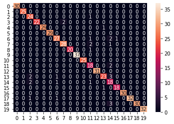
Confusion Matrix

We have an almost perfect confusion matrix on the test dataset, as you can see in Figure 2.

test_pred = label_encoder.inverse_transform(pred)

test_label = label_encoder.inverse_transform(y_test)

cf_matrix = confusion_matrix(test_pred, test_label)

sns.heatmap(cf_matrix, annot=True)

Submission

It’s time to predict on the test database and create our CSV file. This file will be uploaded to the Zindi server for the final score on the hidden test dataset.

sub_pred = model.predict(test_new)

submission = pd.DataFrame()

submission['ID'] = test_data['ID']

submission['Label'] = label_encoder.inverse_transform(sub_pred)

submission.to_csv('submission.csv', index=False)

Conclusion

We got received a bad score on the test dataset. It seems my model is overfitting on both train and validation. This is the best score I got with oversampling, even though my model is overfitting, I got the best result by using SMOTE and SGDClassifier.

I had fun experimenting with various machine learning models from Neural Networks to AutoML, but the dataset was quite small and imbalanced to get a better score.

The winning solution got a 0.7 score.

Focusing on data should be a priority for getting better results. This article was quite simple and beginner-friendly so that anyone can get into the top 50, using my code.

Project Files: GitHub | DAGsHub | Deepnote

About the author

Abid Ali Awan is a certified data scientist professional, who loves building machine learning models and blogging about the latest AI technologies. He is currently testing AI products at PEC-PITC, and recently, he has participated in 60+ competitions, ranging from data analytics to machine learning, to which his creativity in dealing with challenges can be credited to. You can reach him on LinkedIn and Polywork.

Read the original article here.