Côte d’Ivoire Byte-Sized Agriculture Challenge

Helping Côte d'Ivoire
7 000 EUR
Completed (~1 year ago)
Classification
Object Detection
896 joined
163 active
Start
Apr 25, 25
Close
Jun 16, 25
Reveal
Jun 16, 25

🥇 1st Place Solution – Côte d'Ivoire Byte-Sized Agriculture Challenge
Notebooks · 17 Jun 2025, 12:53 · 18
🚜 This solution tackled the challenge of classifying agricultural land use across Côte d'Ivoire using multi-temporal Sentinel-2 imagery (12 bands × 12 months). It combines ConvNeXt for deep spatial-temporal understanding with a LightGBM ensemble boosted by rich handcrafted features.
📌 Final Scores:
- Public LB: 0.973978144
- Private LB: 0.975995377
🔗 Code: GitHub Repo – feel free to ⭐️!
🏗️ Architecture
The solution architecture follows this pipeline:
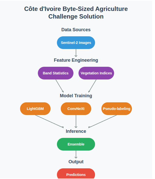
🔍 Summary
🛰 Inputs to convnext model: 144-channel images (12 bands × 12 months)
🌾 Classes: 3 crop types
🧠 Primary Models:
- ConvNeXt-Small (ImageNet-pretrained) – spatial-temporal modeling
- LightGBM – ensemble of vegetation and statistical features
📊 Validation: 15-fold stratified cross-validation
📦 Hardware: Colab Pro – A100 40GB GPU (High RAM)
🔬 Feature Engineering Highlights
- Spectral Band Stats: 8 stats × 12 bands × 12 months = 1,152 features
- Vegetation Indices: 101+ (NDVI, EVI, SAVI, NDWI, etc.) via spyndex
- Temporal Patterns: Month-wise and seasonal aggregations
- Normalization: MinMax scaling with outlier handling
🧪 Training Details
- Image size: 64×64
- Batch size: 32
- Learning rate: 1e-4
- Epochs: 53 (early stopping)
- Augmentations: rotation, flipping, brightness/contrast
🛠️ Reproducibility
- Upload Brainiac_1stPlace_ByteAgriculture_Solution.ipynb to Colab Pro
- Set runtime to A100 40GB + High RAM option
- Run all cells to generate the final_submission.csv
Huge thanks to Zindi and everyone who participated—looking forward to seeing what others cooked up! 👨🏽🌾💡
Brilliant work! Congrats Darius! Well deserved.
Stil new to working with sentinel data. But this notebook is totally enlightening.
Continue the wonderful work!
Appreciate it! Great to hear that the notebook is of help to you.
Convnext base was clearly the outstanding backbone per my small experiments. I did'nt explore >3 channels - would be something worth exploring to see how it stands out. I don't understand your band order - could you kindly explain how you arrived at that?
Lastly, did you attempt object detection using geometry information? if yes , how were your results?
So, for each sample, it contains 12 TIFFs (one per month), and each TIFF has 12 spectral bands—so for a given sample, we have 144 grayscale images total. I treated each unique (month, band) pair as a separate input channel, resulting in a 144-channel input tensor per sample. This structure allows the model to learn both temporal and spectral patterns jointly.
For object detection—I didn’t explore it. The spatial resolution of the images is quite low, which makes precise localization of objects challenging. So I focused on approaches that leverage dense classification instead.
Good work. Calculating band statistics also worked for me a little bit. I am curious though as to how you handled missing tiff files.
Thank you.
For the boosting model (specifically LightGBM), I didn't need to fill the NaNs since it can handle missing values natively.
But for the ConvNeXt-fused model, I filled all NaNs with 999999 to explicitly signal that the data point is out-of-distribution. For missing months, I used blank (zero-filled) images so that each sample consistently had data for all 12 months.
Congrats Darius. I thought metadata and geometry features were not allowed.
Thanks @NogginHq
The metadata and geometry features were only used for EDA and visualization purposes, not for model training or inference. I've updated the notebook to clarify this more explicitly.
Only statistical aggregations and vegetation indices were used
Awesome. Thanks for the clarification.
I just saw this. Finally some notebooks. Let me quickly go through and star this. Congratulations @Brainiac.
Thank you!
Congratulations! How much of a boost did you get from pseudolabeling?
Thank you! Pseudo labelling gave me quite a boost, CV from .96 to .98 and private lb from .95 to .97
That is huge!
Congrats @Brainiac !
I wanted to ask you about the CV-LB consistency, could you tell us about your experience with it?
On our side, our split was based on position + target. Honestly, there was no consistency: our best private score (0.9580) had a public LB of 0.92xx and a CV of 0.94, while our other models were achieving 0.96xx CV.
I noticed you used 15 folds, was there a reason behind this? Did you notice any particular pattern with it?
Thanks! Congrats to you and Muhamed_Tuo as well.
I initially used 10 stratified folds, but the CV–LB correlation wasn’t reliable. I switched to 15 stratified folds based on the assumption that the public LB was around a 25–30% split. With only 282 test samples, 15 folds gave me a closer mimic of that split and improved consistency across CV and LB.
Spectacular 💯. Thanks for the notebook
Thank you! Hope you find it helpful.