Primary competition visual

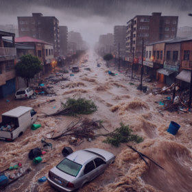
Inundata: Mapping Floods in South Africa

Helping South Africa
$10 000 USD
Completed (~1 year ago)
Classification
1340 joined
315 active
Starti
Nov 22, 24
Closei
Feb 16, 25
Reveali
Feb 17, 25
User avatar
enigmatic
What worked?
Help · 17 Feb 2025, 10:57 · 11

This competition was very interesting and challenging at the same time. I tried heavy feature engineering, undersampling, oversampling, applied images, used several boosting models and adjusted the data(especially when the precipitation was 0 and it was labelled as flood(1) in the train data) but my result was just not improving,

Discussion 11 answers
User avatar
MuhammadQasimShabbeer
Engmatix

same was for me as well Can top ladder postion holder share their insight.

17 Feb 2025, 11:32
Upvotes 0

Summary of the 15th place solution from the private leaderboard:

1. Data Processing

  • Processed multi-band satellite imagery (Blue, Green, Red, NIR, SWIR, Slope)
  • Image resizing and flattening

2. Feature Engineering

  • Time-based features (year, month, day)
  • Precipitation shifts (-300 to +300)
  • Hierarchical statistical aggregations

3. Modeling

  • XGBoost Classifier
  • GPU acceleration
  • StratifiedGroupKFold (5 splits)
  • Group-based prediction normalization
  • Log loss optimization

4. Key Parameters

  • Tree method: hist
  • Device: cuda
  • Scale positive weight: 2
  • Max depth: 5

Kaggle link :

https://www.kaggle.com/code/onurkoc83/floods-study

17 Feb 2025, 13:20
Upvotes 6

Don't forget to upvote the Kaggle notebook :)) , and feel free to ask me if you have any questions.

User avatar
enigmatic

Thank you, great approach! I didn't use many lag and lead features, just previous 20 days and next 21 days.

User avatar
CodeJoe

Will do that🔥. Thanks for sharing.

I will make several videos recap my solutions and what I learned.

Here is the first one: https://www.youtube.com/playlist?list=PLTTjhaP30APfgB-hqzw85olc6w6h8TO43

17 Feb 2025, 15:21
Upvotes 2
User avatar
CodeJoe

Thank you for sharing. We will be very glad on receiving the rest. Big ups!

User avatar
CodeJoe

I was affected by the leak and got a huge shakeup but anyways that's all part of the game😅. This is my solution:

I made 730 lag features (this is for all the days),

Little feature engineering in addition.

The Images didn't help me from my opinion.

Groupkfold of 10 folds,

Xgboost (mostly default parameters, with early stopping and n_estimators of 1000).

Ensemble methods didn't work quite well for me.

This was the score before using the leak:

Public: 0.002575628

Private: 0.002630546

https://www.kaggle.com/code/dukekojokongo/zindi-inundata-floods

18 Feb 2025, 00:11
Upvotes 1

Summary of my Progression and Results:

  1. Rule-based baseline (LB: 0.004810): An initial baseline based on flood days and locations only.
  2. Simple XGBoost baseline (LB: 0.004218): A basic XGBoost model is trained, using the initial features in the dataset without feature engineering.
  3. Add precipitation rolling mean feature (LB: 0.00318): This significant improvement comes from adding rolling mean features of precipitation. The fe function (cv.py, lines 21-45) calculates rolling means for various window sizes (w):for w in list(range(2,100,2)) + list(range(100, 250, 10)): This creates rolling mean features with windows from 2 to 98 (step 2) and 100 to 240 (step 10). These are stored as columns named rm_{w}_precipitation. This captures trends in precipitation over different time scales.
  4. Rolling mean center=True (LB: 0.00296): The center=True argument in the rolling() function within fe (cv.py, line 23) is crucial. Centering the rolling window means that the average at a given time point considers both past and future values. This reduces lag and provides a smoother representation of the precipitation trend.
  5. Add diff and rolling mean of diff (LB: 0.00271): This step adds features related to the change in precipitation. The fe function (cv.py, lines 27-41) calculates lagged differences and their rolling means:df[f'rainfall_lag_{lag}_{col}' = ... .diff(lag).fillna(0): Calculates the difference in precipitation between the current day and lag days prior. fillna(0) handles the initial NaN values. Nested loops create lag_rm_{w}_{lag}_precipitation features. These are rolling means (windows w) of the lagged differences (lag). This captures the trend of precipitation changes over different time scales. This is done for lags of 2, 8, 14, and 28 days, and a variety of window sizes.
  6. Use Gaussian smooth label regression as base margin (LB: 0.00252): This step employs a Gaussian smoothing technique to transform the binary flood labels (0 or 1) into a continuous, "soft" target variable. This smoothed representation is then used as the target variable for an XGBoost regression model. This approach is beneficial because it provides a more nuanced representation of flood risk and helps the model learn a smoother decision boundary. The predictions of this regression model is then used as the base margin for the final classification model
  7. Train image model to classify flood vs non-flood locations and normalize probability (LB: 0.00245): A YOLO image classification model (train_cls.py) is trained to distinguish flood-prone locations. Training uses 128x128 images, data augmentation, and 10 epochs. The model's output probabilities flood_a1 are for each location, which is used to select flood locations and normalize the probabilities.

https://youtu.be/fzPJHU3KYfU?si=mIRRU9JrEqegmerV

18 Feb 2025, 03:01
Upvotes 5
User avatar
enigmatic

Thank you @snow

User avatar
CodeJoe

Well Documented! You deserve a thumbs up. I am definitely subscribing to your channel.