🌱 Introduction: Hundreds Are Better Than One

There’s a popular saying that goes:

“Two heads are better than one.”

But what if you’re not working with two… what if you have hundreds? In the world of machine learning, that’s called an ensemble — and in this case, it’s exactly what led me to the top of the leaderboard.

CodeJoe (Duke Kongo), is an undergraduate student in Ghana and a Data Scientist passionate about turning raw data into powerful insights and practical solutions

Let me, CodeJoe, take you behind the scenes of the Amini Soil Prediction Challenge, a fascinating competition hosted by Zindi and Amini that asked a simple but powerful question:

Can you predict nutrient gaps for a more fertile tomorrow?

Follow along in my GitHub repo.

Soil health is the unsung hero of agriculture. It’s the difference between abundant harvests and food insecurity. In this challenge, the mission was to build a machine learning model that could estimate the availability of 11 essential soil nutrients — macronutrients like Nitrogen (N), Phosphorus (P), and Potassium (K), and micronutrients like Calcium (Ca), Magnesium (Mg), and more.

The goal? Help farmers understand how much of each nutrient is missing for their fields to reach a target maize yield of 4 tons per hectare — a game-changer for optimizing fertilizer use and boosting food production across Africa.

The dataset featured rich environmental data and soil tests from farms across the continent, all collected in 2019. It was a goldmine for any data scientist who enjoys getting their hands dirty (figuratively, of course).

After weeks of deep dives, failed experiments, surprising insights, and some wild ensemble modeling strategies, I was proud to clinch 1st Place on the final leaderboard:

📊 Final Leaderboard Snapshot 🥇 1st Place — CodeJoe (Kwame Nkrumah University of Science and Technology) 🔹 Public Score: 976.05 🔹 Private Score: 1055.17 🔹 Submissions: 237

237 submissions — yeah, you read that right. That’s a lot of trial, error, head-scratching, and “just one more tweak before bed” moments 😅.

The face you make when LightGBM betrays you… again.😭

In this blog, I’ll walk you through the entire journey: from the problem and data to the modeling intuition and final ensemble. Whether you’re new to ML competitions or just love a good under-the-hood story, there’s something here for you.

Let’s dig in. 🧑🏾‍🌾💻

📦 Challenge Overview

The Amini Soil Prediction Challenge, hosted by Zindi in collaboration with Amini, focused on improving soil health insights through machine learning.

🧪 The Objective

Participants were tasked with building a model to predict 11 essential soil nutrients — including Nitrogen (N), Phosphorus (P), Potassium (K), Calcium (Ca), Magnesium (Mg), and more. This was framed as a multi-output regression problem, where each sample required predicting values for all 11 nutrients simultaneously. Whew! That’s a mouthful😅.

Now, what’s multi-output regression? Think of it like trying to guess 11 exam scores for every student — all at once. Instead of training one model per nutrient, multi-output regression lets you predict all 11 at the same time using shared patterns in the data. It’s like one model wearing 11 hats… and trying to balance them without dropping any 🎩🎩🎩🎩🎩🎩🎩🎩🎩🎩🎩.

Makes sense? Maybe? Honestly, let’s just pretend it does and keep moving.

Pretending With Composure😮‍💨

Okay, enough theory — let’s roll up our sleeves and take a look at the dataset itself. 🧑🏾‍🌾📊

🌍 The Dataset

The dataset consisted of:

• 31 features derived from soil samples collected in 2019
• Environmental and satellite data spanning various farms across Africa

These features included geospatial indicators and soil composition data, offering a rich foundation for both exploratory analysis and modeling.

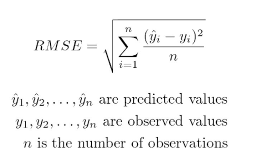
The question is — how did they even know my model was the best? Well, they didn’t just eyeball it and say “this one looks smart.” 😂 An evaluation metric was used to keep things fair and square:

📏 Evaluation Metric

The competition used Root Mean Squared Error (RMSE) to measure how far off each model’s predictions were from the actual nutrient values — across all 11 nutrients. In simple terms, the lower your RMSE, the closer your model was to the truth.

Here’s a quick peek at how RMSE is calculated:

💡My Approach

As the title of this blog suggests, my approach wasn’t just a single model doing all the heavy lifting — it was more like a small army of models working together. In total, I ended up with close to a hundred models, carefully ensembled to squeeze out every bit of predictive power.

But it wasn’t just about throwing models together and hoping for the best. Every piece — from feature engineering to feature selection and even the choice of models — was thoughtfully designed and tested.

To make things easier to follow, I’ve broken down my approach into key sections. First up:

Data Exploration:

One of the best pieces of advice in data science — and one that many of us (myself included 🙈) often skip — is to take EDA seriously. That’s Exploratory Data Analysis, but it definitely sounds cooler as EDA😅.

So, why is EDA important? Here’s what it brings to the table:

• 🧭 Reveals patterns, trends, and hidden issues lurking in your data
• 🧼 Guides your preprocessing decisions, like what to scale, drop, or transform
• 🔍 Helps you visualize relationships between features and the target(s)

During my own EDA, I quickly spotted that Calcium (Ca) was stirring up quite a bit of trouble on the leaderboard. The nutrient’s prediction errors were consistently higher — and when I looked at the distribution of pH values, things started to click. There was a clear pattern that hinted at pH being a major influence on calcium availability.

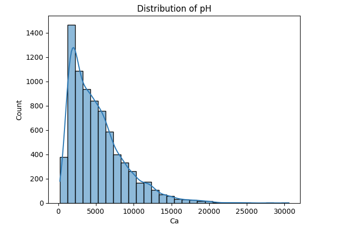
Distribution of pH values in Calcium (Ca).

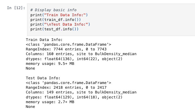
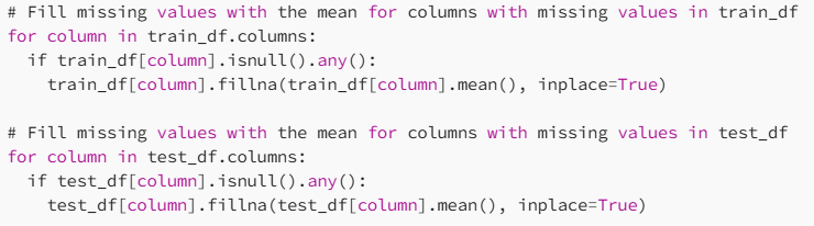
There were several other EDA steps I used as well. To start things off, I ran a quick .info() check using pandas — a simple but powerful way to get a snapshot of the dataset’s structure, including column types and any missing values.

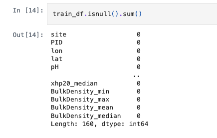
After checking the structure with .info(), my next stop was — you guessed it — missing values. I used df.isnull().sum() to get a quick look at how many values were missing in each column.

Spoiler: there were a few gaps here and there. Nothing too wild, but enough to remind me that even clean-looking datasets can have sneaky holes. I had to decide whether to fill, drop, or ignore — and those decisions can quietly make or break a model. 👀

Display basic info of train and test dataframes.

Oops! Looks like I just dropped a snippet that was supposed to come later. What a spoiler alert 😭! But hey — more on that juicy bit later 😂.

Now, here’s something really interesting: I got a great tip from another participant during the competition who shared his thoughts on the discussion page. A big shoutout to him —Omerym10. He pointed out that the test set contained locations that were much farther off geographically compared to the training set — a detail that could seriously affect model generalization.

And guess what? You wouldn’t catch that kind of insight unless you were doing your due diligence with… you guessed it: EDA!

Yep, good ol’ Exploratory Data Analysis strikes again. 🔍

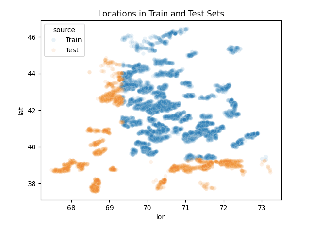
A Snippet From Omerym10 In The Chat on Zindi.

From just these few EDA insights, I started to piece together how I needed to handle the data for my models to actually perform well.

Here’s what I learned early on:

• Never forsake Random Forest 🌲 — especially when outliers are lurking. The wild distribution of pH values for Calcium made this crystal clear. Random Forest handled those quirks like a champ.
• Geo-location matters 📍 — but it’s not just about plugging in latitude and longitude. You’ve got to think about how spatial patterns influence nutrient availability (more on that soon).
• Ensembling is an art 🎨 — and choosing the right combination of models made all the difference.

These early realizations became the backbone of my approach. But let’s not sugarcoat it…

Tears were shed 😭.

Me, after my 10th failed submission for the day thinking I had cracked it. Real ones know this phase.😭

What I was trying just wasn’t working — not at first. There was no golden shortcut or silver platter moment. I had to test, tweak, fail, repeat, over and over again. Feature engineering became a battlefield — but eventually, it became my biggest ally.

Which brings us to… Feature Engineering!

🛠️ Feature Engineering

After EDA gave me some hard truths (and a few tears) on why my previous results were horrible, it was time to turn that insight into action — through features. Because as any data scientist knows:

“Garbage in, garbage out — but magic in, leaderboard clout.” ✨

Here’s what worked, what flopped, and what ultimately helped my models shine:

Before diving deep into the feature engineering magic, let me give you a quick tour of how I structured my overall solution.

I broke it down into five key parts, each building on different ideas and strategies:

1. Extensive Feature Engineering + Random Forest This was the classic tabular setup — lots of handcrafted features and a reliable Random Forest model to get things rolling.
2. Minimal Feature Engineering + Random Forest Sometimes less is more. I wanted to test how a more raw-data-driven Random Forest would perform. (Spoiler: it held its own surprisingly well.)
3. Extensive Feature Engineering + Satellite Data + LightGBM (Log Target) Here, I added LANDSAT-8 satellite data and trained a LightGBM model with log1p-transformed targets, especially to calm Calcium’s wild distribution. This setup used 10-fold cross-validation.
4. Extensive Feature Engineering + Satellite Data + LightGBM (Bayesian Tuned) Similar to part 3, but instead of transforming the target, I kept it raw and introduced Bayesian Optimization for hyperparameter tuning. This was the “Nail in the Coffin” setup — just kidding… but it did hit hard on the leaderboard. 😎
5. The Grand Ensemble Finally, I brought all models in these four sections together in a careful ensemble — blending their strengths and minimizing individual weaknesses.

I’ll be breaking each of these down in more detail soon. But first, let’s zoom into how the features were crafted — the real engine room of this solution.

🧪 Part 1: Extensive Feature Engineering + Random Forest

The first part of my pipeline focused on classic, powerful tabular modeling — no fancy tricks, just solid feature engineering and the ever-reliable Random Forest.

But before anything could happen, I had to address a fundamental issue: Missing values.

Random Forest models in most implementations (like scikit-learn) don’t handle nulls natively — they expect a complete dataset. So my first preprocessing step was to apply:

👉 Mean imputation — simple, effective, and works well for Random Forests, especially when you’re not trying to introduce too much noise through complex imputations.

With that done, I moved on to crafting features from the environmental data: domain-based ratios, pH interactions, and nutrient balance features. This setup gave me a solid baseline, especially for nutrients that behaved “normally” (looking at you, Boron).

Since the data included a site column (grouping samples by location), I realized I could capture additional information about each site by computing summary statistics — things like the minimum, maximum, mean, and median for every numeric feature. Think of it as giving the model a "bird’s eye view" of each site.

Here’s what I did under the hood:

1. 🧹 Excluded irrelevant columns like PID, lon, lat, and the nutrient targets (for training data) to avoid leaking information or cluttering the feature space. I learnt this from our EDA!
2. 🧮 Grouped the data by site_id, then calculated aggregated statistics (min, max, mean, and median) for each numeric feature — giving me a set of rich, site-level descriptors.
3. 🧩 Merged the aggregated features back into the original train_df and test_df, so each sample could benefit from the broader context of its site.

Why did this help? Random Forests love features with clear splits and strong signal. By providing summary statistics for the site, the model could better understand patterns like:

• “Is this sample’s pH high or low compared to the rest of the site?”
• “How does this sample’s organic content compare to the median for the region?”

It’s a simple but powerful form of contextual feature engineering — and it made a noticeable difference in early experiments.

# --- Step 1: Columns to exclude from aggregation ---
exclude_cols = ['PID', 'lon', 'lat', 'site']
agg_cols = [col for col in test_df.columns if col not in exclude_cols and pd.api.types.is_numeric_dtype(test_df[col])]

# --- Step 2: Group by 'site' and compute stats ---
site_stats = test_df.groupby('site')[agg_cols].agg(['min', 'max', 'mean', 'median'])

# Flatten multi-level column names: e.g., pH_mean, pH_std
site_stats.columns = ['_'.join(col).strip() for col in site_stats.columns.values]

# Reset index to merge back with original dataframe
site_stats.reset_index(inplace=True)

# --- Step 3: Merge back to test_df and test_df ---
test_df = test_df.merge(site_stats, on='site', how='left')

# --- Step 1: Columns to exclude from aggregation ---
exclude_cols = ['PID', 'lon', 'lat', 'site', 'N', 'P', 'K', 'Ca', 'Mg', 'S', 'Fe', 'Mn', 'Zn', 'Cu', 'B']
agg_cols = [col for col in train_df.columns if col not in exclude_cols and pd.api.types.is_numeric_dtype(train_df[col])]

# --- Step 2: Group by 'site' and compute stats ---
site_stats = train_df.groupby('site')[agg_cols].agg(['min', 'max', 'mean', 'median'])

# Flatten multi-level column names: e.g., pH_mean, pH_std
site_stats.columns = ['_'.join(col).strip() for col in site_stats.columns.values]

# Reset index to merge back with original dataframe
site_stats.reset_index(inplace=True)

# --- Step 3: Merge back to train_df and train_df ---
train_df = train_df.merge(site_stats, on='site', how='left')

After enriching the data with aggregated site-level features, the next step was to prepare the final feature set for modeling.

First, I dropped irrelevant columns like PID (just an ID), and wp, which didn’t offer predictive value. Then I separated the features (X) from the targets (y), readying the data for training.

But there was one more thing: categorical variables. Some features were of type object or category, and Random Forest (as well as most tree-based models) expects numerical input. So I needed a way to convert them without losing meaning.

Enter: Label Encoding.

To avoid any issues with unseen categories in the test set, I used a smart trick:

• I combined the training and test values for each categorical column before fitting the encoder. This ensured all possible categories were captured.
• Then, I transformed both X and X_test accordingly, assigning each unique category a numeric label.

This step may seem small, but handling categorical variables carefully ensures your model doesn’t panic when it encounters something new during inference. 😉

And just like that, the data was clean, numeric, and ready to be served to the mighty Random Forest model.

from sklearn.preprocessing import LabelEncoder

# Identify categorical columns (assumes object or category types)
categorical_cols = X.select_dtypes(include=['object', 'category']).columns.tolist()

# Apply Label Encoding to each categorical column
label_encoders = {}

for col in categorical_cols:
    le = LabelEncoder()
 
 # Fit on the combined data to handle unseen categories in test set
    combined_data = pd.concat([X[col], X_test[col]], axis=0).astype(str)
    le.fit(combined_data)
 
    X[col] = le.transform(X[col].astype(str))
    X_test[col] = le.transform(X_test[col].astype(str))
 
    label_encoders[col] = le  # Store encoder if you need to inverse transform or reuse

Whew! That was quite the deep dive! 😅 But hey — good feature engineering deserves a little spotlight.

Now that we’ve wrapped up Part 1, let’s keep the momentum going and move on to the next chapter of the journey:

🧪 Part 2: Minimal Feature Engineering + Random Forest

After all the heavy lifting in Part 1, I wanted to see how a more minimalist approach would perform.

This time around, I skipped the bells and whistles. No ratios, no aggregations, no satellite features — just the raw data, with only one essential preprocessing step:

👉 Mean imputation to handle missing values. Simple, clean, and fast.

But there was one critical adjustment I made…

Remember during EDA when we discovered that the test set contained sites that were geographically far off compared to the training set? That could seriously throw off models that overly rely on site.

So in this version, I decided to drop the site column entirely. The idea was to force the model to generalize better, instead of memorizing site-specific patterns that might not show up at test time.

This setup became a kind of baseline sanity check — and to my surprise, even with minimal features, the Random Forest still held its ground reasonably well.

🌍 Part 3: Extensive Feature Engineering + Satellite Data + LightGBM (Log Target)

This part of my solution was where things started to level up. We’re talking remote sensing + boosting power = 🔥

For this notebook, I swapped out Random Forest for LightGBM, which has two big advantages:

• It handles missing values natively — so, no need for mean imputation this time 🧼
• It’s great at capturing complex feature interactions, especially in tabular + satellite combos.

🛰️ Integrating Landsat-8 Data

I introduced Landsat-8 satellite data into the mix — specifically the surface reflectance and thermal bands. But instead of using them raw, I wrote a function to:

1. Aggregate spectral features by site
2. Using multiple stats: mean, std, min, and max
3. Flatten column names for consistency (e.g., SR_B5_mean, ST_B10_max, etc.)
4. Merge the aggregated satellite features back into both the training and test sets

def merge_landsat8_aggregates(train_df, test_df, landsat8_data, pid_col='PID'):
 """
    Aggregates Landsat8 data by PID and merges the aggregated features with train and test DataFrames.

    Parameters:
    - train_df (pd.DataFrame): Training dataframe to merge with Landsat8 features.
    - test_df (pd.DataFrame): Test dataframe to merge with Landsat8 features.
    - landsat8_data (pd.DataFrame): Landsat8 raw data containing 'PID' and spectral bands.
    - pid_col (str): Column to group by (default is 'PID').

    Returns:
    - (pd.DataFrame, pd.DataFrame): Tuple of (train_df_merged, test_df_merged)
    """
 # Define numeric columns for aggregation
    landsat_numeric_cols = [
 'QA_PIXEL', 'QA_RADSAT', 'SR_B1', 'SR_B2', 'SR_B3',
 'SR_B4', 'SR_B5', 'SR_B6', 'SR_B7', 'ST_B10'
    ]

 # Aggregate with multiple statistics
    landsat8_agg = landsat8_data.groupby(pid_col)[landsat_numeric_cols].agg(['mean', 'std', 'min', 'max']).reset_index()

 # Flatten multi-level column names
    landsat8_agg.columns = [f"{col[0]}_{col[1]}" if col[1] else col[0] for col in landsat8_agg.columns.values]

 # Merge with train and test data
    train_merged = train_df.merge(landsat8_agg, on=pid_col, how='left')
    test_merged = test_df.merge(landsat8_agg, on=pid_col, how='left')

 return train_merged, test_merged
train_fe, test_df = merge_landsat8_aggregates(train_fe, test_df, landsat8_data)

This gave the model a much richer view of each sample — combining soil/environmental features with spectral signatures from space. 🚀

🧪 Part 4: Extensive Feature Engineering + Satellite Data + LightGBM (Bayesian Optimized, No Target Scaling)

If Part 3 was the chef’s special, Part 4 was the remix — same ingredients, different spice 🌶️.

In this notebook, I reused everything from Part 3:

• All the extensive feature engineering
• The Landsat-8 satellite features
• The same environmental and soil-based predictors

🤖 Modeling — Why One Model Just Wasn’t Enough

Let’s face it: no single model has all the answers. Some are better with outliers, others love clean distributions. Some thrive on engineered features, while others are satellite data fanatics.

So instead of trying to find one perfect model, I decided to build many imperfect ones — and make them work together. Because as the blog title says: “Hundreds are better than one.” 😎

🎭 Each Model Had a Role to Play

Think of it like a team of specialists:

• Random Forests were my tanky baseline models — they handled noise, outliers, and tabular messiness like pros.
• LightGBM brought speed and sharpness, slicing through large feature spaces and revealing fine-grained patterns.
• Different levels of feature engineering gave each model its own unique lens — one looked closely at interactions, another embraced raw structure.

I wasn’t just ensembling models — I was ensembling perspectives.

🧠 Why Ensembling?

You know that saying: “If you want to go fast, go alone. If you want to go far, go together.” That applies to models, too.

Some models nailed certain nutrients but struggled with others. Some were great at generalization, while others overfit (but knew things others didn’t 👀).

By combining their predictions, I was able to balance their strengths and weaknesses, and reduce variance overall.

Next up: we’ll look at how I validated this diverse cast of models using cross-validation, and why it was critical for leaderboard success. Shall we? 🔄

Perfect! Here’s a clear, well-written explanation for Part 1 of your modeling, highlighting the multi-output regression setup, model choice, and validation — in a way that’s educational and engaging for your readers:

🤖 Modeling — Part 1 and 2: Random Forest for Multi-Output Regression

For both Part 1 and Part 2 of my solution, the task was treated as a classic multi-output regression problem — predicting all 11 soil nutrients simultaneously for each sample.

Instead of training 11 separate models (one per nutrient), I used MultiOutputRegressor to wrap around a single Random Forest Regressor, letting it handle all targets in parallel. This not only simplified the training pipeline but also helped maintain consistency across nutrient predictions.

🔧 Feature Setup

For Part 1, after extensive feature engineering, I did the following:

X = train_df.drop(columns=target_columns + ['PID', 'wp'])

y = train_df[target_columns]

X_test = test_df.drop(columns=['PID', 'wp']) I chose to drop the wp column here because I found it to be uninformative in the presence of other stronger features, and removing it helped reduce noise for the Random Forest.

For Part 2, as said before, I did the following:

X = train_df.drop(columns=target_columns + ['PID', 'site'])
y = train_df[target_columns]
X_test = test_df.drop(columns=['PID', 'site'])

🧪 Train-Validation Split & Model Training

To evaluate model performance before jumping to the leaderboard, I performed a simple 80/20 train-test split:

X_train, X_val, y_train, y_val = train_test_split(X, y, test_size=0.2, random_state=42)

model = MultiOutputRegressor(RandomForestRegressor(n_estimators=50, random_state=42)) model.fit(X_train, y_train)

📈 Validation & Prediction

Once trained, I validated the model on the hold-out set:

The performance wasn’t perfect, but it gave me a solid first look at how well the model could generalize — especially given the large number of targets and wide range of nutrient values.

For test-time predictions:

predictions = model.predict(X_test)

This notebook formed the foundation of my modeling approach — simple, interpretable, and surprisingly effective considering all it had to juggle.

Next up: Part 2, where I strip away the fancy features and see how the raw data holds up on its own 💪.

Perfect! Here’s a clear and reader-friendly write-up you can add right after explaining your model training in Part 1 — explaining how you extracted and visualized feature importances from the multi-output Random Forest.

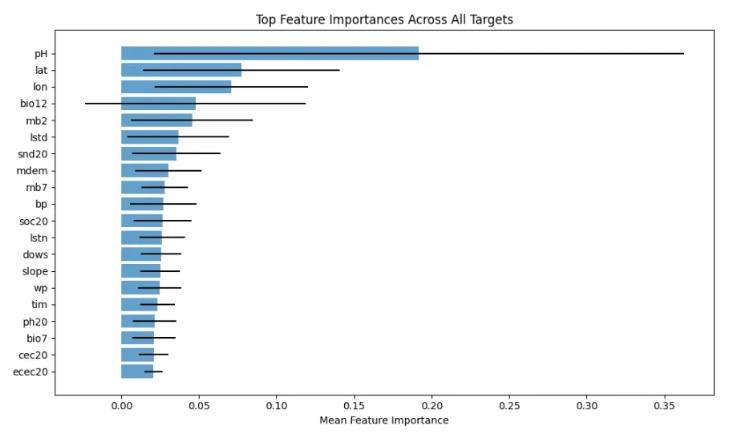
🔍 What Did the Model Care About? (Feature Importances)

Once I trained the Random Forest on all 11 nutrient targets, I was curious — What features were actually doing the heavy lifting?

Since I was using a MultiOutputRegressor, each individual nutrient had its own underlying Random Forest model. That meant I could extract feature importances from each of them, and then calculate the average importance across all targets to get a general view.

Here’s what I did:

# Extract feature importances from each individual regressor
importances = np.array([est.feature_importances_ for est in model.estimators_])

# Aggregate: mean and standard deviation of importance
mean_importances = importances.mean(axis=0)
std_importances = importances.std(axis=0)

I then wrapped these into a DataFrame for easier exploration and plotting:

feature_names = X.columns
importance_df = pd.DataFrame({
    'Feature': feature_names,
    'Mean Importance': mean_importances,
    'Std Dev': std_importances
}).sort_values(by='Mean Importance', ascending=False)

And here’s the fun part: visualizing the top 20 most important features across all nutrient predictions:

plt.figure(figsize=(10, 6))
plt.barh(importance_df['Feature'][:20][::-1], importance_df['Mean Importance'][:20][::-1],
         xerr=importance_df['Std Dev'][:20][::-1], alpha=0.7)
plt.xlabel("Mean Feature Importance")
plt.title("Top Feature Importances Across All Targets")
plt.tight_layout()
plt.show()

This gave me great insights into which features the model consistently relied on — across nutrients — and guided future experiments on what to keep, discard, or transform.

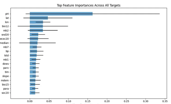
Top Feature Importances Across All Targets for the First Notebook (Random Forest Model).

Top Feature Importances Across All Targets for the Second Notebook (Random Forest Model).

🤖 Modeling — Part 3: LightGBM + Per-Target Models + Satellite Boost!

Okay, this is where things started to get real technical (and real powerful 🚀).

Unlike the earlier notebooks where I used multi-output regression, in this part I decided to train a separate LightGBM model for each nutrient — all 11 of them, one after the other. Why?

Well… not all nutrients behave the same. Some are noisy. Some are chill. Some respond well to log-scaling, some don’t even need it.

So instead of treating them as a group, I gave each nutrient its own custom pipeline — because they deserve love individually 💅.

🏗️ Step 1: Making 11 Custom Datasets

I created 11 versions of the dataset — one for each nutrient — by combining the feature-engineered data (train_fe) with the corresponding target column:

def make_target_dfs(train_fe, train_df, target_columns):
    """
    Creates a dictionary of DataFrames with train_fe plus one target column.

    Args:
        train_fe (pd.DataFrame): DataFrame containing only feature columns.
        train_df (pd.DataFrame): Original DataFrame containing both features and targets.
        target_columns (list): List of target column names to add one at a time.

    Returns:
        dict: Dictionary mapping each target name to a DataFrame with features + that target.
    """
    target_dfs = {}
    for target in target_columns:
        df = train_fe.copy()
        df[target] = train_df[target]
        target_dfs[target] = df
    return target_dfs
target_dfs = make_target_dfs(train_fe, train_df, target_columns)

# Example: Access the DataFrame for 'K'
K_df = target_dfs['K']
N_df = target_dfs['N']
Ca_df = target_dfs['Ca']
P_df = target_dfs['P']
Mg_df = target_dfs['Mg']
Fe_df = target_dfs['Fe']
Mn_df = target_dfs['Mn']
Zn_df = target_dfs['Zn']
Cu_df = target_dfs['Cu']
B_df = target_dfs['B']
S_df = target_dfs['S']

Each DataFrame had:

• All the features
• Just one target (e.g., only K, or only Ca, etc.)

🎯 Step 2: Define X and y for Each Nutrient

From each of these 11 datasets, I created a feature matrix X_ and a target vector y_. I dropped the ID (PID), the water potential (wp), and the target itself to avoid leakage.

Also — log-scaling was applied to most targets using np.log1p (to handle skew), except for Boron (B) which had a nice, clean distribution already.

🧙‍♂️ Step 3: LightGBM Training Spell (with Cross-Validation)

Now for the real magic.

I trained each nutrient’s model using:

• LightGBM
• 10-fold Cross-Validation
• Categorical features handled smartly via .astype("category")
• RMSE as the evaluation metric

Here’s a summary of the setup:

def change_object_to_cat(df):
  # changes objects columns to category and returns dataframe and list

  df = df.copy()
  list_str_obj_cols = df.columns[df.dtypes == "object"].tolist()
  for str_obj_col in list_str_obj_cols:
      df[str_obj_col] = df[str_obj_col].astype("category")

  return df,list_str_obj_cols
X_n, cat_list = change_object_to_cat(X_n)
X_p, cat_list = change_object_to_cat(X_p)
X_k, cat_list = change_object_to_cat(X_k)
X_ca, cat_list = change_object_to_cat(X_ca)
X_mg, cat_list = change_object_to_cat(X_mg)
X_s, cat_list = change_object_to_cat(X_s)
X_fe, cat_list = change_object_to_cat(X_fe)
X_mn, cat_list = change_object_to_cat(X_mn)
X_zn, cat_list = change_object_to_cat(X_zn)
X_cu, cat_list = change_object_to_cat(X_cu)
X_b, cat_list = change_object_to_cat(X_b)

# For Test Set
X_test, cat_list = change_object_to_cat(X_test)

def lgbm_trainer(X_train, y_train, X_test, y_test, params, num_round, categorical):
    """
    Trains an LGBM (LightGBM) model using the training data and evaluates it on the validation data.
    Returns the trained model (bst).
    """

    # Prepare the training dataset for LightGBM
    # 'lgb.Dataset' is used to create a LightGBM dataset object from the training data
    # 'categorical_feature' specifies which columns are categorical
    train_data = lgb.Dataset(X_train, y_train, feature_name=X_train.columns.tolist(), categorical_feature=categorical, free_raw_data=False)

    # Prepare the validation dataset for LightGBM in the same way as the training data
    validation_data = lgb.Dataset(X_test, y_test, feature_name=X_train.columns.tolist(), categorical_feature=categorical, free_raw_data=False)

    # Initialize an empty dictionary to record evaluation results during training
    eval_result = {}

    # Train the LightGBM model using the specified parameters and datasets
    bst = lgb.train(
        params,  # Model parameters (e.g., learning rate, number of leaves, etc.)
        train_data,  # The training dataset
        num_round,  # The number of boosting rounds (iterations)
        valid_sets=[train_data, validation_data],  # Datasets to evaluate during training
        callbacks=[  # Callbacks to use during training            lgb.early_stopping(stopping_rounds=100),  # Stop training early if the validation score doesn't improve for 17 rounds
            lgb.log_evaluation(500),  # Log evaluation results every 100 rounds
            lgb.record_evaluation(eval_result)  # Record evaluation results in 'eval_result'
        ]
    )

    # Return the trained model (bst) after training is complete
    return bst

SEED = 42
# We start by defining default parameters and setting the objective metric
param = {"verbose": -100}  # Set verbosity to -100 to suppress detailed output
param['metric'] = 'rmse'   # Set the evaluation metric to RMSE (Root Mean Squared Error)
param['random_state'] = SEED

# Lists to save metrics and predictions from the cross-validation folds
def cv_train_lgbm(X_train, y_train, params, num_rounds, category):
    """
    Function to perform 14-fold cross-validation and train an LGBM model
    Returns the out-of-fold validation score and the models from the cross-validation
    Parameters:
    X_train (DataFrame): The feature matrix for training.
    y_train (Series): The target labels for training.
    params (dict): The parameters for training the LightGBM model.
    num_rounds (int): The number of boosting iterations (rounds) to train the model.
    cat_list (list): A list of categorical feature names or indices.
    
    Returns:
    tuple: A tuple containing the mean RMSE (float) and the list of trained models (list).
    """
    kf = KFold(n_splits=10, random_state=42, shuffle=True)  # 10-fold cross-validation
    lgbm_rmses = []  # List to store RMSE values for each fold
    lgbm_y_vals = []  # List to store true values for each fold (not used in this example)
    lgbm_y_hats = []  # List to store predicted values for each fold (not used in this example)
    lgbm_models = []  # List to store trained models for each fold

    # Loop through each fold of the cross-validation
    for trn_idx, test_idx in kf.split(X_train, y_train):  # Split the data into training and validation sets
        X_tr, X_val = X_train.iloc[trn_idx], X_train.iloc[test_idx]  # Training and validation features
        y_tr, y_val = y_train.iloc[trn_idx], y_train.iloc[test_idx]  # Training and validation labels
        
        # Train the LGBM model using the training data and validation data
        lgbm_cls = lgbm_trainer(X_tr, y_tr, X_val, y_val, params, num_rounds, category)
        lgbm_models.append(lgbm_cls)  # Save the trained model
        
        # Use the trained model to make predictions on the validation set
        lgbm_y_hat = lgbm_cls.predict(X_val, num_iteration=lgbm_cls.best_iteration)
        
        # Calculate RMSE (Root Mean Squared Error) between true and predicted values
        lgbm_rmse = mean_squared_error(y_val, lgbm_y_hat, squared=False)  # RMSE is the square root of MSE
        lgbm_rmses.append(lgbm_rmse)  # Save the RMSE for this fold
    
    # Calculate the mean RMSE across all folds
    lgbm_mean_rmse = statistics.mean(lgbm_rmses)
    print("Mean RMSE: {}".format(lgbm_mean_rmse))  # Print the average RMSE across all folds
    
    return lgbm_mean_rmse, lgbm_models  # Return the average RMSE and the list of trained models

Each fold trained and evaluated the LightGBM on held-out data, recording the RMSE — and I printed the average at the end.

💡 I kept the LightGBM parameters pretty default, just a few tweaks and a fixed random seed to ensure reproducibility.

📊 Result: One Model to Rule Each Nutrient

Here’s what I got after looping over all 11 nutrients:

for X, y, name in zip(X_list, y_list, target_names):
    print(f"Training for target: {name}")
    rmse, models = cv_train_lgbm(X, y, param, 1000, cat_list)
    models_dict[name.lower()] = models
    rmse_list.append(rmse)

By the end, I had a neat dictionary models_dict containing:

• A list of trained LightGBM models (one per fold) for each nutrient
• RMSE values showing how well they performed individually

And now that each nutrient had its champion, it was time to let them all combine forces… but more on that in Part 5: The Grand Ensemble 🧠🔄.

Great addition! Here’s a polished explanation you can include in your blog to introduce that code block clearly and engagingly:

🌾 Nutrient-by-Nutrient Feature Importance

After training separate LightGBM models for each of the 11 soil nutrients, I wanted to dig deeper — what features mattered the most for each target?

To do this, I used model.feature_importance(importance_type='gain') from LightGBM, which tells us how much each feature contributed to improving the model. Gain importance is a reliable metric because it reflects the actual contribution to loss reduction.

I created a simple function plot_single_model_importance() to visualize the top 35 features for each nutrient. Here's the code and a few key plots:

def plot_single_model_importance(model, feature_names, top_n=20):
    importance = model.feature_importance(importance_type='gain')
    importance_df = pd.DataFrame({
        'feature': feature_names,
        'importance': importance
    }).sort_values(by='importance', ascending=False).head(top_n)

plt.figure(figsize=(10, 6))
    plt.barh(importance_df['feature'], importance_df['importance'], color='green')
    plt.xlabel('Gain Importance')
    plt.title(f'Top {top_n} Feature Importances (Single Model)')
    plt.gca().invert_yaxis()
    plt.tight_layout()
    plt.show()

And then, for each nutrient:

plot_single_model_importance(models_dict['ca'][2], X.columns, top_n=35)
plot_single_model_importance(models_dict['k'][2], X.columns, top_n=35)
plot_single_model_importance(models_dict['mn'][2], X.columns, top_n=35)
plot_single_model_importance(models_dict['cu'][2], X.columns, top_n=35)
plot_single_model_importance(models_dict['b'][2], X.columns, top_n=35)
plot_single_model_importance(models_dict['p'][2], X.columns, top_n=35)
plot_single_model_importance(models_dict['mg'][2], X.columns, top_n=35)
plot_single_model_importance(models_dict['fe'][2], X.columns, top_n=35)
plot_single_model_importance(models_dict['n'][2], X.columns, top_n=35)
plot_single_model_importance(models_dict['zn'][2], X.columns, top_n=35)
plot_single_model_importance(models_dict['s'][2], X.columns, top_n=35)

📌 Pro tip: Doing this nutrient-by-nutrient helped me see which features consistently mattered across nutrients, and which were more specialized. This also gave me ideas on which engineered features were truly worth it.

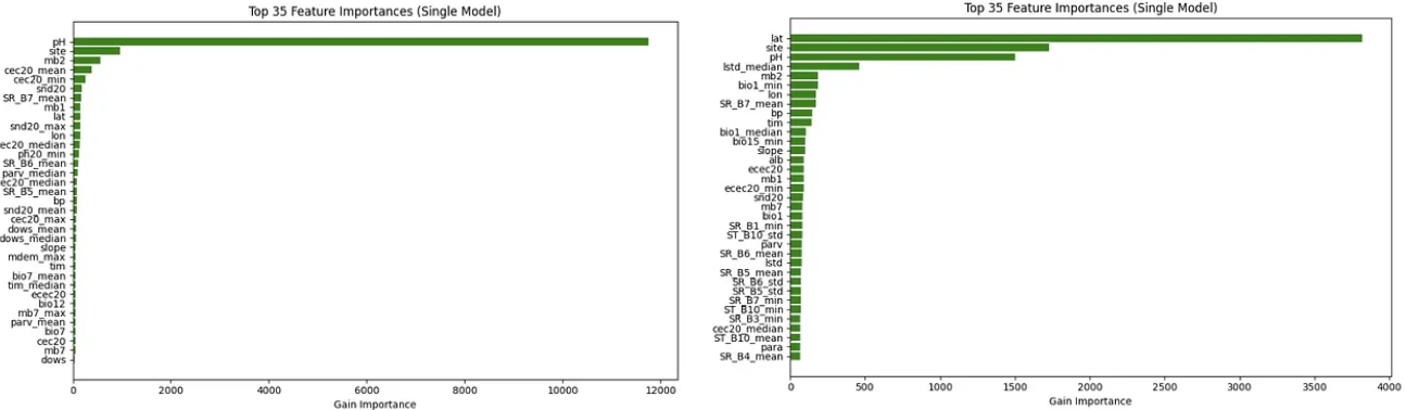
Feature Importances From Calcium (Ca) and Phosphorus (K) on Fold 3.

Here’s a polished and blog-friendly version you can use to explain and introduce this post-processing and prediction blending logic in your Medium article:

🎯 Final Predictions: Median Blending & Nutrient Adjustments

Once the individual LightGBM models for each nutrient were trained and validated, it was time to bring it all together. But instead of relying on just one model’s prediction per nutrient, I used median blending across the 10 folds trained per nutrient.

Why median and not mean? Well, the median is more robust to outliers and noisy folds — which is especially helpful given how wild some nutrient predictions (hello Calcium 👋) could get.

Here’s the code snippet that combines predictions from all models:

# Function to get median prediction from a list of models
def get_mean_prediction(models, X):
    preds = np.array([model.predict(X) for model in models])
    return np.median(preds, axis=0)

Then, for each of the 11 nutrients, I inverse the log transformation (np.expm1) and apply a few nutrient-specific adjustments based on cross-validation insights:

# Get averaged predictions for each target
N_pred  = np.expm1(get_mean_prediction(models_n, X_test)) * 0.95
P_pred  = np.expm1(get_mean_prediction(models_p, X_test))
K_pred  = np.expm1(get_mean_prediction(models_k, X_test))
Ca_pred = np.expm1(get_mean_prediction(models_ca, X_test)) * 1.05  # Boost Calcium a bit
Mg_pred = np.expm1(get_mean_prediction(models_mg, X_test))
S_pred  = np.expm1(get_mean_prediction(models_s, X_test))
Fe_pred = np.expm1(get_mean_prediction(models_fe, X_test))
Mn_pred = np.expm1(get_mean_prediction(models_mn, X_test))
Zn_pred = np.expm1(get_mean_prediction(models_zn, X_test))
Cu_pred = np.expm1(get_mean_prediction(models_cu, X_test))
B_pred  = get_mean_prediction(models_b, X_test)  # No log transform here

📌 Why those nutrient tweaks? I slightly boosted Calcium (Ca) predictions and reduced Nitrogen (N) based on cross-validation behavior and leaderboard feedback. These small nudges added up!

This final prediction stage was crucial — carefully aggregating fold-wise outputs and applying domain-aware nudges made the final submission more robust and leaderboard-ready.

Whew! That was a lot of soil, stats, and sweat 😅. If you’re still reading, you officially deserve a nutrient badge 🏅🌽.

Here’s a clean, reader-friendly write-up for the final notebook in your approach. It builds naturally on the previous sections, emphasizes what’s different, and walks the reader through the training strategy:

🧠 Final Notebook: Full Force LightGBM Stacking (No Log-Transform)

After all the experimentation, I crafted one last notebook — my “all-in” ensemble. It shares the same structure as the previous one (per-target LightGBM training), but with one key twist:

❌ No log1p transformations this time — I let the models learn the raw scale of each nutrient.

Why? Because I wanted to test whether LightGBM, especially when finely tuned, could directly model the nutrient distributions without needing log-smoothing. And spoiler alert: it held up surprisingly well.

🏗️ A Stack of Eight Carefully Tuned LightGBM Models

Instead of training just one LightGBM per nutrient, I trained eight different LightGBM variants — each with its own style:

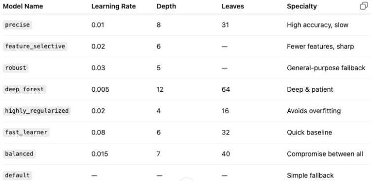
Each of these was trained using 10-fold cross-validation, meaning 80 models per nutrient (8 configs × 10 folds). 🚀 Now do you see where the hundred heads come from😅?

🧪 Bayesian Optimization for Ensemble Weights

After training all 8 models per fold, I didn’t just average their predictions. Instead, I used Bayesian Optimization to find the optimal blend of weights for each fold — automatically learning how much trust to assign each model:

# In each fold, we search for the best weight combo:
def objective_function(**weights):
    w = np.array([weights[f'w{i}'] for i in range(len(model_configs))])
    w = w / np.sum(w)
    pred = np.sum(fold_preds * w, axis=1)
    return -np.sqrt(mean_squared_error(y_val, pred))  # Negative RMSE

This allowed each fold to build a custom ensemble recipe tailored to its data split — kind of like giving each fold its own tasting chef. 👨‍🍳

📉 Final Performance

Once all folds were trained, the final predictions for the test set were obtained by computing the median prediction across folds (again, for robustness):

def get_mean_prediction(stacked_models, X):
    fold_preds = []
    for base_models, weights in stacked_models:
        base_preds = np.array([model.predict(X) for model in base_models])
        weighted_pred = np.average(base_preds, axis=0, weights=weights)
        fold_preds.append(weighted_pred)
    return np.median(fold_preds, axis=0)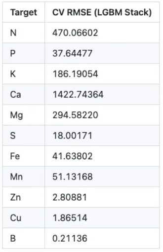

📦 Test-Time Predictions (No log1p reversal this time!)

Here’s the final prediction block for each nutrient:

N_pred  = get_mean_prediction(models_n, X_test)
P_pred  = get_mean_prediction(models_p, X_test)
K_pred  = get_mean_prediction(models_k, X_test)
Ca_pred = get_mean_prediction(models_ca, X_test)
Mg_pred = get_mean_prediction(models_mg, X_test)
S_pred  = get_mean_prediction(models_s, X_test)
Fe_pred = get_mean_prediction(models_fe, X_test)
Mn_pred = get_mean_prediction(models_mn, X_test)
Zn_pred = get_mean_prediction(models_zn, X_test)
Cu_pred = get_mean_prediction(models_cu, X_test)
B_pred  = get_mean_prediction(models_b, X_test)

No reverse log-transform this time — what the model sees is what the model gives. 🎯

🔚 Wrap-Up

This final notebook was like the grand finale in a fireworks show — leveraging all the experimentation, tuning, and insights from earlier notebooks but turning the ensemble dial to eleven.

Did it boost performance? Yep. Especially when paired with smart post-processing and careful ensembling across all notebooks (more on that next 😉).

Whew 😮‍💨… at this point, I won’t lie — I was drained. After wrangling with feature engineering, model tuning, cross-validation, log transforms, and LightGBM stacking for each nutrient… I could practically hear my laptop begging for mercy 😅.

But I wasn’t done yet. There was still one last move on the board — the Ensemble Notebook.

Let’s talk about that final piece of the puzzle 🔗👇.

Sure! Here’s a polished and insightful write-up for your ensemble strategy and scores:

🧮 Notebook Scores (Public Leaderboard / Private Leader board)

To recap, here were the public leaderboard scores for each of the notebooks I created:

• 📘 First notebook (RF with extensive features): 1031.471392 / 1120.745762
• 📙 Second notebook (RF with little features): 1036.39704 / 1147.364051
• 📗 Third notebook (LGBM + log1p + satellite data): 1020.032195 /1110.913702
• 📕 Fourth notebook (LGBM + no log1p + satellite data): 1006.265908 /1064.724457✅

Now, you might be wondering: “Why are you quoting the public leaderboard when Zindi scores us based on the private board?” Well, here’s the thing: we don’t see the private leaderboard until the competition ends. So throughout the challenge, I had to rely on the public scores to gauge progress and tweak my approach.

But let me be clear — this is NOT best practice and I really learnt my lesson from other competitions. Leaderboard probing is risky. Always let your intuition, cross-validation stability, and domain understanding lead the way. The rest? Leave it in God’s hands 😅.

🤝 Final Ensemble Strategy

Once the individual models were trained and validated, it was time to blend them.

Here’s how the ensemble was structured:

# Load predictions
sub1 = pd.read_csv('/kaggle/input/1006-amini-soil-no-log/lgbm_submission_no_log.csv')
sub2 = pd.read_csv('/kaggle/input/1020-amini-soil-lgbm-log-sub/lgbm_submission_log.csv')
sub3 = pd.read_csv('/kaggle/input/amini-soil-random-forest-little-fe-sub/submission-rf_little_fe_postprocess.csv')
sub4 = pd.read_csv('/kaggle/input/random-forest-sub-extensive-fe-amini-soil/submission-rf_extensive_fe.csv')

# Blend LightGBM models (Notebook 3 & 4)
lgbm_sub = sub1.copy()
lgbm_sub.Gap = (sub1.Gap * 0.5) + (sub2.Gap * 0.5)
# Blend Random Forest models (Notebook 1 & 2)
rf_sub = sub3.copy()
rf_sub.Gap = (sub3.Gap * 0.5) + (sub4.Gap * 0.5)
# Final blend: LGBM (65%) + RF (35%)
final_sub = lgbm_sub.copy()
final_sub.Gap = ((lgbm_sub.Gap * 0.65) + (rf_sub.Gap * 0.35))

🧠 Why 65/35?

The fourth notebook (LGBM with no log transform) had the best public score and best private score (1064.724457) with the strongest CV stability — so it naturally formed the core of the final blend.

However, sub3 (RF with minimal features) performed surprisingly well in some nutrient-specific evaluations. Giving Random Forest models a 35% voice in the final prediction:

• Injected diversity
• Smoothed out potential overfitting from LGBM
• Gave credit to simpler models that often generalize better

The result? A balanced, robust ensemble that played it safe — and ultimately led to my best private leaderboard score on Zindi. 🏆

🔹 Public Score: 976.05 🔹 Private Score: 1055.17

Now, on to reflections and key takeaways!

🔍 Key Reflections

Let’s take a final look at how each notebook performed — both publicly and privately:

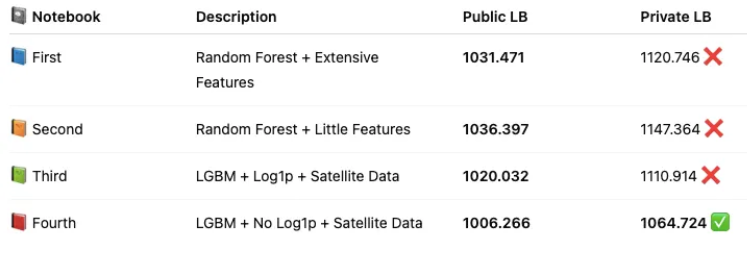
Looking at the private leaderboard, you can clearly see the shake-up — models that seemed strong on the public board didn’t always hold up privately.

So what saved the day?

✨ Ensembling.

Blending models gave my solution:

• Greater robustness
• Lower risk of overfitting to public leaderboard quirks
• A way to balance out the biases of individual models

💡 Final Thought

“Hundreds will always be better than one.”

In a competition setting where you can’t see the private board, playing it safe with diverse models is a smart move.

In the real world? You don’t get to probe a hidden test set either. That’s why techniques like:

• Cross-validation,
• Blending,
• And model diversity…

…are not just competition tricks — they’re best practices.

So yes, probe when you can, but trust your validation and intuition, ensemble wisely, and when all else fails — leave the rest in God’s hands 😅

Now that’s a wrap! 🏁

Recap on Painful Moments😭:

Me thinking I was cooking… but the leaderboard said ‘burnt offering’ 😭🔥

🙏 Thank You!

To everyone who made it this far — thank you for reading through my journey, experiments, and painful struggles😭. This competition taught me more than just modeling; it taught me persistence, humility, and the beauty of iteration.

If you’d like to explore the code, notebooks, and more behind the scenes:

🔗 Check out my GitHub here

Feel free to star the repo, raise issues, or just say hi! I’m always open to feedback and collaboration.

About Me

I'm Duke Kojo Kongo, a Data Scientist passionate about turning raw data into powerful insights and practical solutions. With a strong foundation in Python, SQL, and machine learning, I’ve built models across domains—from credit scoring to sales forecasting—delivering both accuracy and business value.

On Zindi, I’ve competed in a variety of challenges that push the limits of data science, constantly learning and adapting along the way. My mission is to build data-driven tools that are not only technically sound but also impactful in real-world settings, especially in the African context where innovation can truly change lives.