Lacuna Solar Survey Challenge

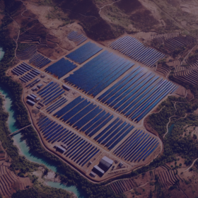
Can you identify solar panels and boilers in satellite and drone imagery?

1.Dataset

1.1.Initial analysis revealed annotation flaws including:

· Polygon misalignment

· Partially omitted panels ("pans")

· Incorrect panel numbering ("pan_nbr")

1.2.We addressed these by:

· Converting polygon annotations to DOTA format

· Performing data cleaning and relabeling using LabelImg2 (custom fork with rotated box support), but we used CoCo format finally

2.Key Insight

2.1.Object detection (vs. direct regression) proves more effective for:

· Precise localization of solar panels/boilers

· Accurate counting in Madagascar's satellite/drone imagery

3.Data Preprocessing

3.1.Domain Separation Strategy:

· Original image sources D (4000×3000/5280×3920) and S (600×600) exhibit significantly different resolutions

· Model cannot learn cross-domain features effectively (risk of interference)

· Final approach: Train separate models for D and S domains

3.2.Data Filtering:

· Removed ambiguous images with mismatch between actual counts and annotated numbers

3.3.Data Split:

· Creating 2 or more folds and insuring that the distribution of val contains extreme values (pan_nbr > 100) with equal distribution

4.Model Selection on D

Model

Epochs

Performance Notes

YOLO11m (RTX 4080 16G)

300 (72 hours)

Baseline performance, ultimately discarded.

DDQ (2*T4 2*16G)

14 + 10 (24hours)

Optimal convergence & accuracy

Co DINO (A10G 24G)

14 (12 hours)

Optimal convergence & accuracy

4.1.Why DDQ and Co DINO Wins:

1. 10× faster convergence (24 epochs vs 300 epochs)

2. Superior performance on:

• Dense object clusters
• Small object detection (critical for satellite imagery)
• Occlusion handling

4.2. Training methods

We constructed two distinct datasets with strategic validation splits to address extreme-value distributions (panel numbers exceeding 100). Both datasets maintained balanced extreme-value representation across training and validation sets (train₁-val₁ and train₂-val₂). Independent models were trained on each configuration, with final predictions derived through ensembled outputs.

4.3. Data augmentation

· Random Horizontal/Vertical Flip: RandomFlip with probability 0.5.

· Color Jitter: ColorJitter with brightness/contrast/saturation (±20%) and hue (±10%) adjustments.

· CLAHE (Contrast-Limited Adaptive Histogram Equalization): Enhances contrast with clip limit 2.0 and grid size 8x8.

· Gaussian Blur: Blurs images with sigma range 0.1-2.0.

· Random Affine Transformations: Scaling: 0.9-1.1x/Translation: ±10% shift/Rotation: ±20 degrees.

· Random Brightness/Contrast: Adjusts brightness/contrast (±30%) with 30% probability.

· Image Sharpening: Sharpens edges with alpha 0.1-0.3 and lightness 0.75-1.5x.

· Multi-scale Pipeline:Resize to 1280x1280 (keep ratio)/Resize → Random0Crop (384x640) → Resize to 1280x1280.

4.4. Threshold Optimization Strategy

For images containing a high density of solar panels (defined as >100 panels per image in this study), we observed systematic under-detection due to overly conservative confidence thresholds.

We implemented a dual-phase adjustment:

1. Confidence thresholds tuning: Minimized MAE loss on the validation set for general threshold calibration.

2. High-density specialization: Empirically reduced the confidence threshold to 0.1 exclusively for images where preliminary detections exceeded 100 panels.

4.5. Location-Optimized Ensemble Strategy

Experimental analysis reveals varied model performance across installation locations. The complete DDQ architecture underperforms on rooftop imagery compared to alternative models. We therefore implement an adaptive weighting system that strategically combines model strengths by deployment position.

Ensemble weights were established through validation evaluation, with an exception: Fold 2 model's ambiguous validation performance prompted provisional low-weight assignment. Leaderboard validation confirmed this configuration's effectiveness, justifying its retention.

5.Model Selection on S

Model

Epochs

Performance Notes

YOLO11m (RTX 4080 16G)

300 (2 hours x 5 folds)

Baseline performance

5.1.Data augmentation:

· resize to 1024

· random rotate / multi_scale / translate / flip v,h / mosaic / mixup / cos_lr

· training on 5 folds

5.2.Test Time Augment

· Pan: SAHI get sliced prediction for 450x450 slice, considering the smaller size of pan

· Boil: multi_scales prediction on 876(1, 0.86, 1.3)

· Model ensemble to get mean pan_nbr and boil_nbr

Model

Epochs

Performance Notes

DINO (P100 16G)

37 (24hours)

Optimal convergence & accuracy

DDQ (P100 16G)

14 (12hours)

Optimal convergence & accuracy

5.3.Data augmentation:

· Multi-scale resizing

· Random horizontal flipping (50% probability)

· Color space normalization

· PhotoMetricDistortion (contrast/brightness/saturation/hue adjustments)

5.4.Weighted Ensemble Strategy

Blends DINO, DDQl, and YOLO results at different weight

6.Process:

📷

7.Winning Edges:

• We recognized the poor annotation quality of the dataset and manually corrected and annotated them
• Instead of approaching it as a prediction task, we framed it as an object detection task, which enhanced accuracy and interpretability
• We selected powerful DETR-series models (DDQ, DINO), which significantly outperformed the YOLO-series models
• Multiple TTA, post-processing, ensemble strategies were employed to address various potential scenarios, achieving a lower MAE